Spatial Modelling with Composable Gaussian Processes#
Download this notebook: spatial_linear_gp.ipynb
This notebook shows how to construct a semiparametric linear model by composing a linear model in NumPyro with a GPJax Gaussian Process (GP). We build two components: firstly, the linear component which ncodes a global affine trend with Bayesian linear regression. We then define a GP residual component which is responsible for capturing spatial structure that the linear term’s residual.
The example highlights the interplay between GPJax and NumPyro: GPJax provides the GP
prior and likelihood definitions, whilst NumPyro performs Hamiltonian Monte Carlo (HMC)
inference across all parameters in a unified model and allows us to draw upon a broader set of
modelling components. If you have not seen the two libraries used together before, the
NumPyro integration notebook sets out the mechanics on a
simpler model than this one.
Data Simulation#
We simulate a 2D spatial dataset (\(N=200\)) on a domain \([0, 5] \times [0, 5]\). The generative process contains a linear trend: \(y_{\text{lin}} = 2x_1 - 1x_2 + 1.5\) with an additive spatial residual: \(y_{\text{res}} = \sin(x_1) \cos(x_2)\). To this, we add simulate an additive homoscedastic noise component \(\epsilon \sim \mathcal{N}(0, 0.1^2)\). The dominant linear trend masks a non-linear residual. Composing models lets us represent both behaviours without forcing a single mechanism to fit every feature of the data.
from functools import partial

import jax
import jax.numpy as jnp
import jax.random as jr
import matplotlib as mpl
import matplotlib.pyplot as plt
import numpyro
import numpyro.distributions as dist
from numpyro.infer import (
    MCMC,
    NUTS,
    Predictive,
)

from utils import use_mpl_style
import gpjax as gpx

jax.config.update("jax_enable_x64", True)

use_mpl_style()
cols = mpl.rcParams["axes.prop_cycle"].by_key()["color"]


N = 200
key = jr.key(123)
keys = jr.split(key, 8)

X = jr.uniform(keys[0], shape=(N, 2), minval=0.0, maxval=5.0)

# True Linear Trend
true_slope = jnp.array([2.0, -1.0])
true_intercept = 1.5
y_lin = X @ true_slope + true_intercept

# Non-linear Spatial Residual
y_res = jnp.sin(X[:, 0]) * jnp.cos(X[:, 1])

# Total Signal + Noise
latent_signal = y_lin + y_res
noise_stddev = 0.1
y = latent_signal + noise_stddev * jr.normal(keys[1], shape=latent_signal.shape)
Linear Component#
We begin by defining a Bayesian linear regression model in NumPyro. This component will later be combined with a GP residual, but for now, we’ll establish a baseline model through ordinary linear regression.
We use the No-U-Turn Sampler (NUTS) to draw samples from the posterior distributions of the slope \(\mathbf{w}\), intercept \(b\), and noise \(\sigma\).
def linear_model(X, Y=None):
    slope = numpyro.sample("slope", dist.Normal(0.0, 5.0).expand([2]))
    intercept = numpyro.sample("intercept", dist.Normal(0.0, 5.0))
    obs_noise = numpyro.sample("obs_noise", dist.LogNormal(0.0, 1.0))

    mu = X @ slope + intercept
    numpyro.deterministic("mu", mu)
    numpyro.sample("obs", dist.Normal(mu, obs_noise), obs=Y)


nuts_kernel_lin = NUTS(linear_model)
mcmc_lin = MCMC(
    nuts_kernel_lin,
    num_warmup=50 if ci else 1500,
    num_samples=50 if ci else 2000,
    num_chains=1,
)
mcmc_lin.run(keys[2], X, y)
mcmc_lin.print_summary()
                 mean       std    median      5.0%     95.0%     n_eff     r_hat
  intercept      1.37      0.11      1.37      1.22      1.53     15.96      1.07
  obs_noise      0.49      0.02      0.50      0.44      0.51     12.10      1.09
   slope[0]      2.07      0.03      2.07      2.03      2.13     45.27      1.01
   slope[1]     -1.03      0.03     -1.03     -1.08     -1.00     21.04      1.01

Number of divergences: 0
Composing the Linear Component with a GP#
We now augment the linear component with a GP tasked with modelling the residual.
GPJax and NumPyro Integration#
We define the GP prior in GPJax using a second-order
Matérn kernel and a
constant mean function
(since the linear trend is handled explicitly). The
introduction to kernels describes the Matérn family and the
smoothness each member assumes. Hyperparameters are sampled
directly with numpyro.sample and passed to the GPJax constructors as raw JAX arrays.
We then compute the exact marginal log-likelihood (MLL) of the residuals under the GP
prior using gpx.objectives.conjugate_mll — the
same objective optimised in the
regression notebook, here contributed to a NumPyro model instead.
This term is added to the potential function using numpyro.factor, guiding the sampler.
def joint_model(X, Y, X_new=None):
    slope = numpyro.sample("slope", dist.Normal(0.0, 5.0).expand([2]))
    intercept = numpyro.sample("intercept", dist.Normal(0.0, 5.0))

    lengthscale = numpyro.sample("lengthscale", dist.LogNormal(0.0, 1.0))
    variance = numpyro.sample("variance", dist.LogNormal(0.0, 1.0))
    obs_noise = numpyro.sample("obs_noise", dist.LogNormal(0.0, 1.0))

    kernel = gpx.kernels.Matern32(
        active_dims=[0, 1], lengthscale=lengthscale, variance=variance
    )
    meanf = gpx.mean_functions.Constant()
    gp_prior = gpx.gps.Prior(mean_function=meanf, kernel=kernel)
    likelihood = gpx.likelihoods.Gaussian(obs_stddev=obs_noise)
    gp_posterior = gp_prior * likelihood

    trend = X @ slope + intercept

    if Y is not None:
        residuals = Y - trend
        residuals = residuals.reshape(-1, 1)
        D_resid = gpx.Dataset(X=X, y=residuals)
        mll = gpx.objectives.conjugate_mll(gp_posterior, D_resid)
        numpyro.factor("gp_log_lik", mll)

    if X_new is not None:
        if Y is not None:
            residuals = Y - trend
            residuals = residuals.reshape(-1, 1)
            D_resid = gpx.Dataset(X=X, y=residuals)

            latent_dist = gp_posterior.predict(X_new, train_data=D_resid)
            f_new = numpyro.sample("f_new", latent_dist)
            f_new = f_new.reshape((-1, 1))

            total_prediction = (X_new @ slope + intercept).reshape(-1, 1) + f_new
            numpyro.deterministic("y_pred", total_prediction)


joint_model_wrapper = joint_model
nuts_kernel_joint = NUTS(joint_model_wrapper)
# In practice, one should run more samples from multiple chains.
mcmc_joint = MCMC(
    nuts_kernel_joint,
    num_warmup=50 if ci else 1500,
    num_samples=50 if ci else 2000,
    num_chains=1,
)
mcmc_joint.run(keys[3], X, y)
mcmc_joint.print_summary()
                   mean       std    median      5.0%     95.0%     n_eff     r_hat
    intercept      1.50      1.26      1.65     -0.56      3.72     18.42      1.01
  lengthscale      4.13      0.96      3.97      3.10      6.17      9.64      1.05
    obs_noise      0.11      0.01      0.11      0.10      0.12     33.40      0.98
     slope[0]      1.87      0.24      1.85      1.55      2.10     23.15      1.01
     slope[1]     -0.95      0.22     -0.96     -1.25     -0.60     48.03      0.98
     variance      1.55      1.18      1.15      0.42      3.55      8.66      1.12

Number of divergences: 0
Comparison and Visualization#
We evaluate the linear model in isolation, and then the joint model where a GP has been included to model the residual.
samples_lin = mcmc_lin.get_samples()
predictive_lin = Predictive(linear_model, samples_lin, return_sites=["mu"])
preds_lin = predictive_lin(keys[4], X=X)["mu"]
mean_pred_lin = jnp.mean(preds_lin, axis=0)

samples_joint = mcmc_joint.get_samples()
predictive_joint = Predictive(
    joint_model_wrapper, samples_joint, return_sites=["y_pred"]
)
preds_joint = predictive_joint(keys[5], X=X, Y=y, X_new=X)["y_pred"]
mean_pred_joint = jnp.mean(preds_joint, axis=0)

rmse_lin = jnp.sqrt(jnp.mean((mean_pred_lin.flatten() - latent_signal.flatten()) ** 2))
rmse_joint = jnp.sqrt(
    jnp.mean((mean_pred_joint.flatten() - latent_signal.flatten()) ** 2)
)

print("\nRMSE Comparison (vs True Signal):")
print(f"Linear Model: {rmse_lin:.4f}")
print(f"Joint Model:  {rmse_joint:.4f}")
RMSE Comparison (vs True Signal):
Linear Model: 0.4761
Joint Model:  0.0443
Let’s now plot the predicted profiles from both models (Fig. 37).
n_grid = 30
x1 = jnp.linspace(0, 5, n_grid)
x2 = jnp.linspace(0, 5, n_grid)
X1, X2 = jnp.meshgrid(x1, x2)
X_grid = jnp.column_stack([X1.ravel(), X2.ravel()])

y_grid_true = (X_grid @ true_slope + true_intercept) + (
    jnp.sin(X_grid[:, 0]) * jnp.cos(X_grid[:, 1])
)

preds_lin_grid = predictive_lin(keys[6], X=X_grid)["mu"]
mean_pred_lin_grid = jnp.mean(preds_lin_grid, axis=0)

preds_joint_grid = predictive_joint(keys[7], X=X, Y=y, X_new=X_grid)["y_pred"]
mean_pred_joint_grid = jnp.mean(preds_joint_grid, axis=0)

fig, axes = plt.subplots(1, 3, figsize=(12, 3), sharey=True)

vmin = min(y_grid_true.min(), mean_pred_lin_grid.min(), mean_pred_joint_grid.min())
vmax = max(y_grid_true.max(), mean_pred_lin_grid.max(), mean_pred_joint_grid.max())
levels = jnp.linspace(vmin, vmax, 20)

c0 = axes[0].tricontourf(
    X_grid[:, 0], X_grid[:, 1], y_grid_true, levels=levels, cmap="magma"
)
axes[0].set_title("True Signal")

c1 = axes[1].tricontourf(
    X_grid[:, 0],
    X_grid[:, 1],
    mean_pred_lin_grid.flatten(),
    levels=levels,
    cmap="magma",
)
axes[1].set_title(f"Linear Model (RMSE: {rmse_lin:.2f})")

c2 = axes[2].tricontourf(
    X_grid[:, 0],
    X_grid[:, 1],
    mean_pred_joint_grid.flatten(),
    levels=levels,
    cmap="magma",
)
axes[2].set_title(f"Joint Model (RMSE: {rmse_joint:.2f})")

cbar = fig.colorbar(c0, ax=axes.tolist())
cbar.ax.yaxis.set_major_formatter(mpl.ticker.FormatStrFormatter("%d"))

for ax in axes:
    ax.set_xlabel("x1")
    ax.scatter(X[:, 0], X[:, 1], c=cols[0], s=10, alpha=0.5)
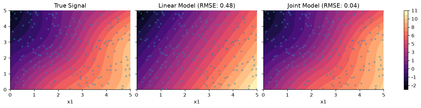
Fig. 37 The true signal alongside the posterior mean surface of the linear model and of the joint linear-plus-GP model, with the observation locations overlaid.#
System configuration#
%load_ext watermark
%watermark -n -u -v -iv -w -a "Thomas Pinder"
Author: Thomas Pinder

Last updated: Fri, 25 Sep 2026

Python implementation: CPython
Python version       : 3.11.16
IPython version      : 9.17.1

gpjax     : 0.18.0
jax       : 0.10.2
matplotlib: 3.11.2
numpyro   : 0.21.0

Watermark: 2.6.0