Dual Parameterisation of Sparse GPs (t-SVGP)#
Download this notebook: dual_svgp.ipynb
This applied companion to the natural gradients notebook checks the dual (site) parameterisation of Adam et al. [2021] in GPJax. Read that notebook for the derivation; here we compare implementation and theory on conjugate regression, matched site/moment steps, a three-optimiser classification benchmark, and M-step bound slices and variational EM (VEM). natgrads.py focuses on the moment-storage branch.
Below, \(\boldsymbol{\theta}\) denotes kernel hyperparameters, while \(\boldsymbol{\lambda}=(\boldsymbol{\lambda}_1,\boldsymbol{\Lambda}_2)\) denotes the stored sites; \(\mathbf{a}_i = \mathbf{K}_{zz}^{-1}\mathbf{k}_z(x_i)\).
# Enable Float64 for more stable matrix inversions.
import time

import equinox as eqx
import jax
from jax import config
import jax.numpy as jnp
import jax.random as jr
from jaxtyping import install_import_hook
import matplotlib as mpl
import matplotlib.pyplot as plt
import optax as ox
import paramax
from utils import clean_legend, use_mpl_style

config.update("jax_enable_x64", True)


with install_import_hook("gpjax", "beartype.beartype"):
    import gpjax as gpx
    import gpjax.kernels as jk
    from gpjax.natural_gradients import (
        natural_gradient_step,
        partition_variational,
    )
    from gpjax.objectives import dual_elbo, elbo
    from gpjax.parameters import Real, val
    from gpjax.variational_families import (
        DualVariationalGaussian,
        VariationalGaussian,
    )

key = jr.key(123)

# set the default style for plotting
use_mpl_style()
cols = mpl.rcParams["axes.prop_cycle"].by_key()["color"]


def negative_elbo(model, data):
    """The loss for a family that stores moments; GPJax optimisers descend."""
    return -elbo(model, data)


def negative_dual_elbo(model, data):
    """The loss for a family that stores sites."""
    return -dual_elbo(model, data)
What DualVariationalGaussian stores#
The family stores the unnormalised Gaussian site multiplying the prior:
Its moments are \(\mathbf{S}=(\mathbf{K}_{zz}^{-1}+
\boldsymbol{\Lambda}_2)^{-1}\) and \(\mathbf{m}=\boldsymbol{\mu}_z+
\mathbf{S}\boldsymbol{\lambda}_1\). dual_vector and dual_matrix
store the flanked, precision sites
\((\boldsymbol{\lambda}_1,\boldsymbol{\Lambda}_2)\); zero sites initialise
\(q=p\). For each likelihood term, the update uses
One jax.grad call on expected_log_likelihood supplies both.
For Gaussian observations, compare it with the closed form
\(\alpha_i=(y_i-m_i)/\sigma^2\), \(\beta_i=1/\sigma^2\):
key, alpha_beta_key = jr.split(key)
check_response = jr.normal(alpha_beta_key, (5, 1))
check_mean = jnp.linspace(-1.0, 1.0, 5)
check_variance = jnp.linspace(0.2, 0.9, 5)
check_stddev = 0.37
check_likelihood = gpx.likelihoods.Gaussian(obs_stddev=check_stddev)


def total_expected_log_likelihood(mean, variance):
    """Summed variational expectation, as a function of the marginal moments."""
    return jnp.sum(
        check_likelihood.expected_log_likelihood(
            check_response, mean[:, None], variance[:, None]
        )
    )


bonnet_alpha, price_derivative = jax.grad(
    total_expected_log_likelihood, argnums=(0, 1)
)(check_mean, check_variance)
price_beta = -2.0 * price_derivative

closed_form_alpha = (check_response.squeeze(-1) - check_mean) / check_stddev**2
closed_form_beta = jnp.full_like(check_mean, 1.0 / check_stddev**2)

print(
    "max |alpha - (y - m) / sigma^2| : "
    f"{jnp.max(jnp.abs(bonnet_alpha - closed_form_alpha)):.3e}"
)
print(
    "max |beta - 1 / sigma^2|        : "
    f"{jnp.max(jnp.abs(price_beta - closed_form_beta)):.3e}"
)
max |alpha - (y - m) / sigma^2| : 1.066e-14
max |beta - 1 / sigma^2|        : 4.441e-15
Both derivatives match the Gaussian closed form; the natural gradients notebook derives how these per-point terms become the tied sites.
Gaussian regression: one step to the optimum#
For Gaussian observations, the site targets are independent of \(q\):
Thus \(\rho=1\) reaches the fixed point in one step, yielding
The resulting moments are the Titsias [2009] optimum. The non-zero mean below checks that sites act on the centred process.
num_data = 200
noise_stddev = 0.3
observation_variance = noise_stddev**2
prior_constant = 0.4
regression_lengthscale = 0.5
regression_jitter = 1e-8

key, input_key, noise_key = jr.split(key, 3)
regression_inputs = jr.uniform(input_key, (num_data, 1), minval=-3.0, maxval=3.0)
regression_outputs = jnp.sin(2.0 * regression_inputs) + noise_stddev * jr.normal(
    noise_key, (num_data, 1)
)
regression_data = gpx.Dataset(X=regression_inputs, y=regression_outputs)

num_inducing = 20
regression_inducing = jnp.linspace(-3.0, 3.0, num_inducing).reshape(-1, 1)


def conjugate_model(lengthscale):
    """The conjugate joint model (prior * likelihood) at a given RBF lengthscale."""
    prior = gpx.gps.Prior(
        mean_function=gpx.mean_functions.Constant(jnp.array(prior_constant)),
        kernel=jk.RBF(lengthscale=lengthscale),
        jitter=regression_jitter,
    )
    return prior * gpx.likelihoods.Gaussian(obs_stddev=noise_stddev)


def site_family(lengthscale, inducing_inputs, sites=None):
    """A dual family, optionally carrying a frozen pair of sites."""
    family = DualVariationalGaussian(
        model=conjugate_model(lengthscale),
        inducing_inputs=inducing_inputs,
    )
    if sites is None:
        return family
    return eqx.tree_at(
        lambda tree: (tree.dual_vector, tree.dual_matrix),
        family,
        (Real(sites[0]), Real(sites[1])),
    )


def moment_family(lengthscale, inducing_inputs, moments):
    """A moment family carrying a frozen $(m, S)$."""
    mean, covariance = moments
    return VariationalGaussian(
        model=conjugate_model(lengthscale),
        inducing_inputs=inducing_inputs,
        variational_mean=mean,
        variational_root_covariance=jnp.linalg.cholesky(covariance),
    )


def exact_sites(lengthscale, inducing_inputs, dataset):
    """One rho = 1 conjugate step from lambda = 0: the exactly optimal sites."""
    variational, hyper = partition_variational(
        site_family(lengthscale, inducing_inputs)
    )
    variational, _ = natural_gradient_step(
        variational, hyper, dataset, negative_dual_elbo, 1.0
    )
    fitted = eqx.combine(variational, hyper)
    return (val(fitted.dual_vector), val(fitted.dual_matrix)), fitted.moments()
# The Titsias optimum in closed form, against the same jittered K_zz the family uses.
initial_dual = site_family(regression_lengthscale, regression_inducing)
regression_prior = initial_dual.model.prior
regression_kernel = regression_prior.kernel
regression_mean_function = regression_prior.mean_function

Kzz = regression_kernel.gram(regression_inducing).as_matrix()
Kzz = Kzz + regression_jitter * jnp.eye(num_inducing)
Kzx = regression_kernel.cross_covariance(regression_inducing, regression_inputs)
centred_outputs = regression_outputs - regression_mean_function(regression_inputs)

titsias_precision = Kzz + Kzx @ Kzx.T / observation_variance
optimal_mean = (
    regression_mean_function(regression_inducing)
    + Kzz
    @ jnp.linalg.solve(titsias_precision, Kzx @ centred_outputs)
    / observation_variance
)
optimal_covariance = Kzz @ jnp.linalg.solve(titsias_precision, Kzz)

# The collapsed (Titsias) bound, which the dual ELBO must reproduce at that optimum.
nystrom = Kzx.T @ jnp.linalg.solve(Kzz, Kzx)
marginal_covariance = nystrom + observation_variance * jnp.eye(num_data)
_, marginal_logdet = jnp.linalg.slogdet(marginal_covariance)
marginal_quadratic = centred_outputs.squeeze(-1) @ jnp.linalg.solve(
    marginal_covariance, centred_outputs.squeeze(-1)
)
prior_variance_diagonal = jnp.diag(
    regression_kernel.gram(regression_inputs).as_matrix()
)
sparsity_gap = jnp.sum(prior_variance_diagonal - jnp.diag(nystrom)) / (
    2 * observation_variance
)
collapsed_bound = (
    -0.5 * (num_data * jnp.log(2 * jnp.pi) + marginal_logdet + marginal_quadratic)
    - sparsity_gap
)
# One dual natural-gradient step at rho = 1, from lambda = 0.
dual_variational, dual_hyper = partition_variational(initial_dual)
stepped_variational, _ = natural_gradient_step(
    dual_variational, dual_hyper, regression_data, negative_dual_elbo, 1.0
)
stepped_dual = eqx.combine(stepped_variational, dual_hyper)
stepped_mean, stepped_covariance = stepped_dual.moments()

# A second step must be a no-op.
twice_stepped_variational, _ = natural_gradient_step(
    stepped_variational, dual_hyper, regression_data, negative_dual_elbo, 1.0
)
twice_stepped_dual = eqx.combine(twice_stepped_variational, dual_hyper)
twice_stepped_mean, twice_stepped_covariance = twice_stepped_dual.moments()

stepped_bound = dual_elbo(stepped_dual, regression_data)

print(f"dual_elbo after one step    : {float(stepped_bound):12.6f}")
print(f"Titsias collapsed bound     : {float(collapsed_bound):12.6f}")
print(
    f"max |m - m*|                : {jnp.max(jnp.abs(stepped_mean - optimal_mean)):.3e}"
)
print(
    "max |S - S*|                : "
    f"{jnp.max(jnp.abs(stepped_covariance - optimal_covariance)):.3e}"
)
fixed_point_gap = max(
    jnp.max(jnp.abs(twice_stepped_mean - stepped_mean)),
    jnp.max(jnp.abs(twice_stepped_covariance - stepped_covariance)),
)
print(f"max fixed-point moment change : {fixed_point_gap:.3e}")
print(f"collapsed bound - dual_elbo : {float(collapsed_bound - stepped_bound):.12e}")
print(
    "N * jitter / (2 sigma^2)    : "
    f"{num_data * regression_jitter / (2 * observation_variance):.12e}"
)
dual_elbo after one step    :   -82.659588
Titsias collapsed bound     :   -82.659577
max |m - m*|                : 3.489e-12
max |S - S*|                : 2.139e-13
max fixed-point moment change : 2.487e-14
collapsed bound - dual_elbo : 1.111111103569e-05
N * jitter / (2 sigma^2)    : 1.111111111111e-05
The first step matches the closed-form moments, and a second step leaves
them unchanged. The small difference from the analytic collapsed bound
is \(N\varepsilon/(2\sigma^2)\): Prior.jitter adds \(\varepsilon\) to each
predictive marginal variance in GPJax’s ELBO, but not to the formula
for the collapsed bound above.
This agreement does not imply that the constant
\(c(\boldsymbol{\theta})\) relating the dual bound to a site
log-partition function vanishes. For normalised projected sites it is
minus the Titsias trace term (sparsity_gap), non-zero for sparse
\(\mathbf{Z}\ne\mathbf{X}\). For GPJax’s unnormalised flanked sites the
normaliser changes the constant too. GPJax evaluates the bound as a
variational expectation minus KL instead.
Matched site and moment steps#
The site and moment steps agree when all computed \(\beta_i\geq 0\).
To see where beta_floor changes that identity, we take six matched
\(\rho=\gamma=0.8\) steps on the banana classification data used in the
natural gradients notebook. A run without clipping
isolates its effect before we compare longer optimisation trajectories.
def make_banana(key, num_points):
    """Two-class banana problem with a curved Bayes-optimal boundary."""
    key_latent, key_label = jr.split(key)
    latent = jr.uniform(key_latent, (num_points, 2), minval=-3.0, maxval=3.0)
    decision = latent[:, 1] - (0.7 * latent[:, 0] ** 2 - 1.5)
    probability = jax.nn.sigmoid(3.0 * decision)
    labels = (jr.uniform(key_label, (num_points,)) < probability).astype(jnp.float64)
    return latent, labels[:, None]


banana_key = jr.key(42)
banana_inputs, banana_labels = make_banana(banana_key, 2000)
banana_data = gpx.Dataset(X=banana_inputs, y=banana_labels)

num_train = 1600
train_inputs, test_inputs_2d = banana_inputs[:num_train], banana_inputs[num_train:]
train_labels, test_labels = banana_labels[:num_train], banana_labels[num_train:]
banana_train = gpx.Dataset(X=train_inputs, y=train_labels)

num_banana_inducing = 50
inducing_grid = jnp.meshgrid(jnp.linspace(-2.8, 2.8, 10), jnp.linspace(-2.8, 2.8, 5))
banana_inducing = jnp.stack([axis.ravel() for axis in inducing_grid], axis=1)
banana_jitter = 1e-6

banana_model = (
    gpx.gps.Prior(
        mean_function=gpx.mean_functions.Zero(),
        kernel=jk.RBF(active_dims=[0, 1]),
    )
    * gpx.likelihoods.Bernoulli()
)

banana_gram = banana_model.prior.kernel.gram(
    banana_inducing
).as_matrix() + banana_jitter * jnp.eye(num_banana_inducing)
banana_prior_root = jnp.linalg.cholesky(banana_gram)


def make_banana_moment_family():
    """A fresh SVGP over the banana data, at q = p."""
    return VariationalGaussian(
        model=banana_model,
        inducing_inputs=banana_inducing,
        variational_mean=jnp.zeros((num_banana_inducing, 1)),
        variational_root_covariance=banana_prior_root,
    )


print(f"Train / test: {banana_train.n} / {banana_data.n - banana_train.n}")
Train / test: 1600 / 400
def implied_moments(family):
    """Return $(m, S)$ for either parameterisation."""
    if isinstance(family, DualVariationalGaussian):
        return family.moments()
    root = val(family.variational_root_covariance)
    return val(family.variational_mean), root @ root.T


def price_curvature(family, data):
    """Compute $\\beta_i=-2\\,\\partial_{v_i}E_q[\\log p]$."""
    marginal_mean, marginal_variance = family.marginals(data.X)

    def total_expectation(variance):
        return jnp.sum(
            family.model.likelihood.expected_log_likelihood(
                data.y, marginal_mean[:, None], variance[:, None]
            )
        )

    return -2.0 * jax.grad(total_expectation)(marginal_variance)


def six_matched_steps(beta_floor):
    """Six rho = 0.8 steps in both branches, from the shared q = p start."""
    site_partition, site_hyper = partition_variational(
        DualVariationalGaussian(
            model=banana_model,
            inducing_inputs=banana_inducing,
        )
    )
    moment_partition, moment_hyper = partition_variational(make_banana_moment_family())
    rows = []
    for _ in range(6):
        # Check curvature at the current site iterate, before updating it.
        curvature = price_curvature(
            eqx.combine(site_partition, site_hyper), banana_train
        )
        site_partition, _ = natural_gradient_step(
            site_partition,
            site_hyper,
            banana_train,
            negative_dual_elbo,
            0.8,
            beta_floor=beta_floor,
        )
        moment_partition, _ = natural_gradient_step(
            moment_partition, moment_hyper, banana_train, negative_elbo, 0.8
        )
        site_mean, site_covariance = implied_moments(
            eqx.combine(site_partition, site_hyper)
        )
        moment_mean, moment_covariance = implied_moments(
            eqx.combine(moment_partition, moment_hyper)
        )
        rows.append(
            (
                max(
                    float(jnp.max(jnp.abs(site_mean - moment_mean))),
                    float(jnp.max(jnp.abs(site_covariance - moment_covariance))),
                ),
                int(jnp.sum(curvature < 0)),
            )
        )
    return rows


matched_rows = six_matched_steps(1e-8)
print("step   |(m, S) gap|   beta < 0")
for step, (gap, negative_count) in enumerate(matched_rows, start=1):
    print(f"{step:4d}   {gap:12.3e}   {negative_count:4d}/{banana_train.n}")

unfloored_gap = max(gap for gap, _ in six_matched_steps(-jnp.inf))
print(f"Worst gap without clipping: {unfloored_gap:.3e}")
step   |(m, S) gap|   beta < 0
   1      7.305e-14      0/1600
   2      1.170e-13      0/1600
   3      9.459e-14      0/1600
   4      2.638e-13      0/1600
   5      1.717e-03      1/1600
   6      5.104e-03      1/1600
Worst gap without clipping: 3.251e-13
The branches agree to float64 precision until a negative \(\beta_i\) appears; then clipping separates their moments. Without clipping, the gap stays near the noise floor through all six steps. Thus later trajectory differences need not imply a different E-step direction: the clip and, when hyperparameters move, the M-step both matter.
Banana classification: three optimisers#
We compare Adam alone with moment and site natural gradients. All start at \(q=p\) over the same inducing grid; timings exclude JIT compilation.
banana_dual_family = DualVariationalGaussian(
    model=banana_model,
    inducing_inputs=banana_inducing,
)
natgrad_family = make_banana_moment_family()
adam_family = make_banana_moment_family()

# As in the natural-gradients notebook, ramp the step rate from 1e-4 to 1e-1.
num_iterations = 1000
batch_size = 256
natgrad_schedule = ox.exponential_decay(
    init_value=1e-4, transition_steps=100, decay_rate=1000.0, end_value=1e-1
)


def timed_fit(run):
    """Run twice: the first call pays JIT compilation, the second is steady state."""
    model, history = run()
    history.block_until_ready()
    start = time.perf_counter()
    model, history = run()
    history.block_until_ready()
    return model, history, time.perf_counter() - start


shared_settings = dict(
    train_data=banana_train,
    optim=ox.adam(1e-2),
    batch_size=batch_size,
    num_iters=num_iterations,
    key=jr.key(1),
    verbose=False,
)
dual_model, dual_history, dual_seconds = timed_fit(
    lambda: gpx.fit_natgrads(
        model=banana_dual_family,
        objective=negative_dual_elbo,
        natgrad_lr=natgrad_schedule,
        **shared_settings,
    )
)
natgrad_model, natgrad_history, natgrad_seconds = timed_fit(
    lambda: gpx.fit_natgrads(
        model=natgrad_family,
        objective=negative_elbo,
        natgrad_lr=natgrad_schedule,
        **shared_settings,
    )
)
adam_model, adam_history, adam_seconds = timed_fit(
    lambda: gpx.fit(model=adam_family, objective=negative_elbo, **shared_settings)
)

for name, seconds in [
    ("t-SVGP (dual) + Adam", dual_seconds),
    ("natural gradients + Adam", natgrad_seconds),
    ("Adam only", adam_seconds),
]:
    print(
        f"{name:26s}: {seconds:5.2f} s "
        f"({1e3 * seconds / num_iterations:.2f} ms / iteration)"
    )
t-SVGP (dual) + Adam      :  4.86 s (4.86 ms / iteration)
natural gradients + Adam  :  4.47 s (4.47 ms / iteration)
Adam only                 :  2.84 s (2.84 ms / iteration)
smoothing_window = 25


def smooth(history):
    """Trailing mean over `smoothing_window` iterations."""
    return jnp.convolve(
        history, jnp.ones(smoothing_window) / smoothing_window, mode="valid"
    )


smoothed_iterations = jnp.arange(smoothing_window - 1, num_iterations)
curves = [
    ("t-SVGP (dual) + Adam", smooth(dual_history), dual_seconds, cols[2]),
    ("Natural gradients + Adam", smooth(natgrad_history), natgrad_seconds, cols[1]),
    ("Adam only", smooth(adam_history), adam_seconds, cols[0]),
]

elbo_floor = 0.95 * min(float(curve.min()) for _, curve, _, _ in curves)
elbo_ceiling = 1.10 * max(float(curve.max()) for _, curve, _, _ in curves)

fig, axes = plt.subplots(ncols=2, figsize=(10, 3.0), sharey=True)
for name, curve, seconds, colour in curves:
    axes[0].plot(smoothed_iterations, curve, color=colour, label=name)
    axes[1].plot(
        jnp.linspace(0.0, seconds, num_iterations)[smoothing_window - 1 :],
        curve,
        color=colour,
        label=name,
    )
axes[0].set(xlabel="Iteration", yscale="log", ylim=(elbo_floor, elbo_ceiling))
axes[1].set(xlabel="Wall-clock seconds", yscale="log", ylim=(elbo_floor, elbo_ceiling))
axes[0].set_ylabel("Negative ELBO (mini-batch)")
clean_legend(axes[0])
clean_legend(axes[1])

for name, curve, seconds, _ in curves:
    print(f"{name:26s}: negative ELBO {float(curve[-1]):8.2f} after {seconds:.2f} s")
t-SVGP (dual) + Adam      : negative ELBO   306.21 after 4.86 s
Natural gradients + Adam  : negative ELBO   299.22 after 4.47 s
Adam only                 : negative ELBO   322.00 after 2.84 s
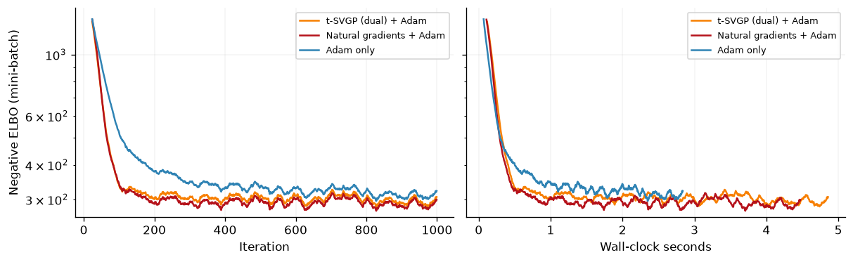
Both natural-gradient runs improve faster than Adam here, whether measured by iteration or wall-clock time. The dual and moment steps cost about the same per iteration at \(M=50\), \(B=256\): avoiding an \(\mathcal{O}(M^3)\) round trip need not dominate the \(\mathcal{O}(BM^2)\) marginal computations. These CPU timings do not test the larger, multi-latent setting of Adam et al. [2021].
The two natural-gradient curves diverge substantially despite their
matched E-step directions before clipping. fit_natgrads also updates
kernel hyperparameters and inducing inputs with Adam, using dual_elbo
for sites and elbo for moments. Their hyperparameter gradients can
differ away from an optimal E-step; the ramping step rate keeps these
E-steps incomplete early on. The dual run finishes at a higher (worse)
negative ELBO on this seed. Because the hyperparameters and inducing
inputs then differ, that result does not rank the M-step objectives.
Next we hold the variational state or the inducing inputs fixed to
examine those objectives more directly.
The M-step in practice#
In an M-step, elbo holds the variational moments fixed as the kernel
changes; dual_elbo holds the data-derived sites fixed, allowing the
prior contribution to \(q\) to track \(\mathbf{K}_{zz}(\boldsymbol{\theta})\).
At an optimal E-step they agree in value and gradient; away from it,
their gradients can differ. See the
natural gradients notebook for the proof.
First we vary a single kernel lengthscale with each representation
frozen, then compare the objectives in a VEM loop.
log_offsets = jnp.linspace(-1.2, 0.6, 61)
frozen_sites, frozen_moments = exact_sites(
    regression_lengthscale, regression_inducing, regression_data
)


def bound_slice(inducing_inputs, dataset, sites, moments, offsets):
    """`dual_elbo` and `elbo` along a log-lengthscale slice, at frozen q."""
    dual_values, moment_values = [], []
    for offset in offsets:
        lengthscale = regression_lengthscale * jnp.exp(offset)
        dual_values.append(
            dual_elbo(site_family(lengthscale, inducing_inputs, sites), dataset)
        )
        moment_values.append(
            elbo(moment_family(lengthscale, inducing_inputs, moments), dataset)
        )
    return jnp.array(dual_values), jnp.array(moment_values)


dual_slice, moment_slice = bound_slice(
    regression_inducing, regression_data, frozen_sites, frozen_moments, log_offsets
)

fig, axes = plt.subplots(ncols=2, figsize=(10, 3.0))
axes[0].plot(log_offsets, dual_slice, color=cols[2], label=r"$\bar l$ (dual_elbo)")
axes[0].plot(log_offsets, moment_slice, color=cols[1], label=r"$l$ (elbo)")
axes[0].axvline(0.0, color="black", linestyle="--", linewidth=1)
axes[0].set(
    xlabel=r"$\Delta\log\ell$ from $\theta_t$",
    ylabel="Bound (nats)",
    ylim=(float(dual_slice.min()) - 40.0, float(dual_slice.max()) + 10.0),
    title=f"Sparse, $M = {num_inducing}$",
)
clean_legend(axes[0])

for inducing_count, colour in [(5, cols[0]), (10, cols[3]), (20, cols[2])]:
    sparse_inducing = jnp.linspace(-3.0, 3.0, inducing_count).reshape(-1, 1)
    sparse_sites, sparse_moments = exact_sites(
        regression_lengthscale, sparse_inducing, regression_data
    )
    sparse_dual, sparse_moment = bound_slice(
        sparse_inducing, regression_data, sparse_sites, sparse_moments, log_offsets
    )
    gap = sparse_dual - sparse_moment
    axes[1].plot(log_offsets, gap, color=colour, label=f"$M = {inducing_count}$")
    print(
        f"M = {inducing_count:2d}: minimum dual-minus-standard gap "
        f"{float(gap.min()):+.3e}"
    )
axes[1].axhline(0.0, color="black", linestyle="--", linewidth=1)
axes[1].set(
    xlabel=r"$\Delta\log\ell$ from $\theta_t$",
    ylabel=r"$\bar l - l$ (nats)",
    yscale="symlog",
    title="Dominance is not uniform when sparse",
)
clean_legend(axes[1])
M =  5: minimum dual-minus-standard gap -2.668e-01
M = 10: minimum dual-minus-standard gap -3.276e-01
M = 20: minimum dual-minus-standard gap -1.421e-14
<Axes: title={'center': 'Dominance is not uniform when sparse'}, xlabel='$\\Delta\\log\\ell$ from $\\theta_t$', ylabel='$\\bar l - l$ (nats)'>
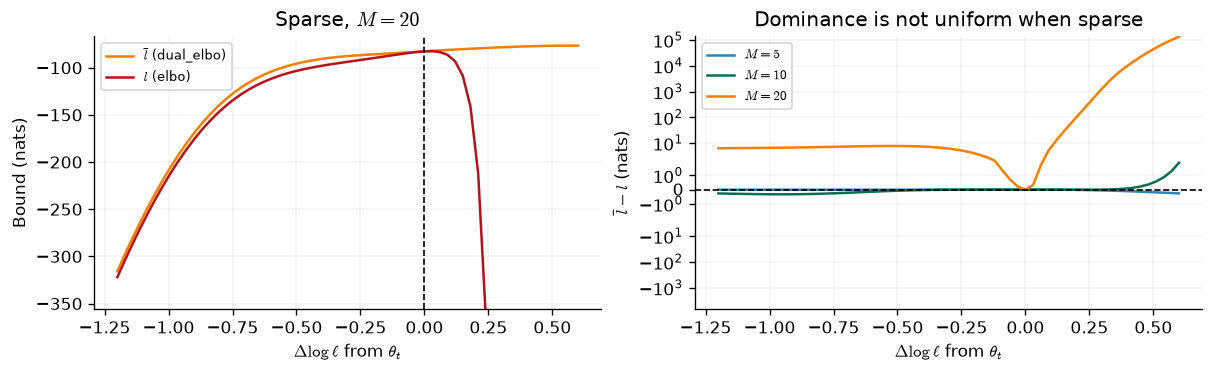
Left: the bounds meet at the E-step optimum
\(\boldsymbol{\theta}_t\). As lengthscale increases, freezing the
moments makes elbo fall sharply, while dual_elbo changes more slowly
because its prior contribution follows the kernel. In the opposite
direction both bounds deteriorate with the sparse approximation.
Right: for \(M=20\) the dual bound is higher across this slice (up to numerical noise at the shared point), but for \(M=5\) and \(M=10\) the gap becomes negative. The dominance guarantee for \(\mathbf{Z}=\mathbf{X}\) does not cover arbitrary sparse inducing sets.
A bound slice is not a training result. To compare M-steps, we now
alternate the same natural-gradient E-step (apart from beta_floor)
with Adam updates on either objective. We fix the inducing inputs so
only the kernel lengthscale moves, starting from a short lengthscale.
expectation_steps = 20
maximisation_steps = 5
vem_rounds = 40
vem_rate = 0.5
vem_optimiser = ox.adam(5e-2)
initial_lengthscale = 0.25


def freeze_inducing(model):
    """Hold the inducing inputs still, so the M-step moves only the kernel."""
    return eqx.tree_at(
        lambda tree: tree.inducing_inputs,
        model,
        paramax.non_trainable(model.inducing_inputs),
    )


def vem_joint_model(lengthscale):
    return (
        gpx.gps.Prior(
            mean_function=gpx.mean_functions.Zero(),
            kernel=jk.RBF(active_dims=[0, 1], lengthscale=lengthscale),
            jitter=banana_jitter,
        )
        * gpx.likelihoods.Bernoulli()
    )


vem_gram = vem_joint_model(initial_lengthscale).prior.kernel.gram(
    banana_inducing
).as_matrix() + banana_jitter * jnp.eye(num_banana_inducing)

vem_dual = freeze_inducing(
    DualVariationalGaussian(
        model=vem_joint_model(initial_lengthscale),
        inducing_inputs=banana_inducing,
    )
)
vem_moments = freeze_inducing(
    VariationalGaussian(
        model=vem_joint_model(initial_lengthscale),
        inducing_inputs=banana_inducing,
        variational_mean=jnp.zeros((num_banana_inducing, 1)),
        variational_root_covariance=jnp.linalg.cholesky(vem_gram),
    )
)


def run_vem(model, objective):
    """Alternate `expectation_steps` E-steps with `maximisation_steps` M-steps."""
    variational, hyper = partition_variational(model)
    opt_state = vem_optimiser.init(eqx.filter(hyper, eqx.is_array))

    @eqx.filter_jit
    def expectation_step(variational, hyper):
        def body(carry, _):
            updated, _ = natural_gradient_step(
                carry, hyper, banana_train, objective, vem_rate
            )
            return updated, None

        return jax.lax.scan(body, variational, None, length=expectation_steps)[0]

    @eqx.filter_jit
    def maximisation_step(variational, hyper, opt_state):
        def hyper_loss(hyper):
            return objective(eqx.combine(variational, hyper), banana_train)

        def body(carry, _):
            hyper, opt_state = carry
            loss, gradient = eqx.filter_value_and_grad(hyper_loss)(hyper)
            updates, opt_state = vem_optimiser.update(
                gradient, opt_state, eqx.filter(hyper, eqx.is_array)
            )
            return (eqx.apply_updates(hyper, updates), opt_state), loss

        (hyper, opt_state), losses = jax.lax.scan(
            body, (hyper, opt_state), None, length=maximisation_steps
        )
        return hyper, opt_state, losses[-1]

    lengthscales, bounds = [], []
    for _ in range(vem_rounds):
        variational = expectation_step(variational, hyper)
        hyper, opt_state, loss = maximisation_step(variational, hyper, opt_state)
        combined = eqx.combine(variational, hyper)
        lengthscales.append(float(val(combined.model.prior.kernel.lengthscale)))
        bounds.append(float(loss))
    return eqx.combine(variational, hyper), jnp.array(lengthscales), jnp.array(bounds)


dual_vem_model, dual_lengthscales, dual_bounds = run_vem(vem_dual, negative_dual_elbo)
moment_vem_model, moment_lengthscales, moment_bounds = run_vem(
    vem_moments, negative_elbo
)
fig, axes = plt.subplots(ncols=2, figsize=(10, 3.0))
rounds = jnp.arange(1, vem_rounds + 1)
for name, lengthscales, colour in [
    ("M-step on dual_elbo", dual_lengthscales, cols[2]),
    ("M-step on elbo", moment_lengthscales, cols[1]),
]:
    axes[0].plot(rounds, lengthscales, color=colour, label=name)
axes[0].set(xlabel="VEM round", ylabel=r"Lengthscale $\ell$")
clean_legend(axes[0])

# The two bound traces are visually identical at this scale, so plot their difference:
# positive means the dual M-step is the further down the negative ELBO of the two.
bound_lead = moment_bounds - dual_bounds
axes[1].plot(rounds, bound_lead, color=cols[2])
axes[1].axhline(0.0, color="black", linestyle="--", linewidth=1)
axes[1].set(
    xlabel="VEM round",
    ylabel="Bound lead to dual_elbo (nats)",
    title="Lead of the dual M-step over the standard one",
)


def test_metrics(model):
    """Held-out accuracy and negative log predictive density."""
    probability = model.model.likelihood(model(test_inputs_2d)).mean
    labels = test_labels.ravel()
    log_density = jnp.mean(
        labels * jnp.log(probability) + (1.0 - labels) * jnp.log1p(-probability)
    )
    return float(jnp.mean((probability > 0.5) == (labels > 0.5))), float(-log_density)


for name, model, lengthscales, bounds in [
    ("dual_elbo", dual_vem_model, dual_lengthscales, dual_bounds),
    ("elbo     ", moment_vem_model, moment_lengthscales, moment_bounds),
]:
    accuracy, nlpd = test_metrics(model)
    print(
        f"M-step on {name}: lengthscale {float(lengthscales[-1]):.4f}, "
        f"negative ELBO {float(bounds[-1]):8.3f}, "
        f"test accuracy {accuracy:.4f}, test NLPD {nlpd:.4f}"
    )
M-step on dual_elbo: lengthscale 1.4127, negative ELBO  295.759, test accuracy 0.9300, test NLPD 0.1626
M-step on elbo     : lengthscale 1.3636, negative ELBO  296.601, test accuracy 0.9300, test NLPD 0.1625
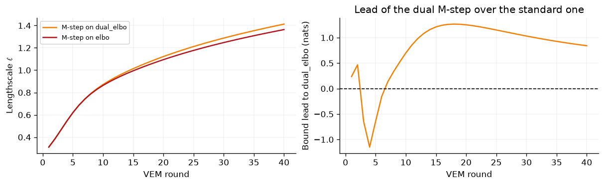
The lengthscale trajectories separate after several rounds. The bound
lead in the right panel is not uniformly positive: the dual branch
falls behind early, then finishes with a modestly better bound and a
longer lengthscale. Held-out accuracy and predictive log density are
similar. This shows different paths under incomplete E-steps, not a
general speed-up or a guarantee that dual_elbo wins.
This is one seed, one kernel hyperparameter and fifty fixed inducing inputs, not the large multi-latent setting of Adam et al. [2021]. The M-step mechanism is narrower: when the E-step is incomplete, keeping sites fixed gives a different hyperparameter gradient from keeping moments fixed.
Caveats#
One latent process. The tied projection used here assumes a latent-diagonal variational family; multi-output models need their own site structure.
Computed curvature matters. A non-log-concave likelihood can give \(\beta_i<0\), threatening positive semidefiniteness. Even GPJax’s Bernoulli likelihood can do so in its tails because
inv_probitclips probabilities.beta_floor(default \(10^{-8}\)) floors the computed \(\beta_i\), keeping the dual update in the PSD cone but breaking exact \(\rho=\gamma\) equivalence with the moment step, as seen above.Keep \(\rho\in(0,1]\). Beyond one, the update extrapolates past a locally valid target and loses its convex-combination guarantee.
fit_natgradsrejects larger constant rates for this family.Flanked sites can be ill-conditioned. Their conditioning scales with \(\operatorname{cond}(\mathbf{K}_{zz})^2\) even when the moments and bound remain accurate; see the numerical demonstration in the natural gradients notebook.
No better E-step direction. At fixed \(\boldsymbol{\theta}\), the dual step gives the same \(q\) as the moment natural gradient when \(\beta_i\geq0\); differences here arise from clipping, runtime, or the M-step objective, not a superior search direction.
System configuration#
%reload_ext watermark
%watermark -n -u -v -iv -w -a 'Thomas Pinder'
Author: Thomas Pinder

Last updated: Fri, 25 Sep 2026

Python implementation: CPython
Python version       : 3.11.16
IPython version      : 9.17.1

equinox   : 0.13.8
gpjax     : 0.18.0
jax       : 0.10.2
jaxtyping : 0.3.11
matplotlib: 3.11.2
optax     : 0.2.8
paramax   : 0.0.5

Watermark: 2.6.0