Natural Gradients

Download this notebook: natural_gradients.ipynb

This notebook is the prerequisite for two others: the natural gradients notebook and the dual sparse GP notebook. Between them those two cover the GPJax API — how to call gpx.fit_natgrads, how to choose a variational family, how the method behaves on real training runs — and they assume everything below already: the exponential-family geometry of \(q(\mathbf{u})\), the identity that makes the natural gradient free to compute, the site/dual reparameterisation of that same geometry, and the guarantees and failure modes attached to both. Read this one first; the other two will not re-derive any of it.

Variational inference in a sparse Gaussian process asks us to optimise a probability distribution \(q(\mathbf{u})\), not a point in \(\mathbb{R}^P\). Gradient descent does not know that: it moves the storage coordinates of \(q\) — a mean vector and a Cholesky factor, or, as we will see, a pair of site parameters — as though they lived in flat Euclidean space, and so the step it takes depends on how we happened to write the distribution down. The natural gradient repairs this by measuring distance between distributions with the Fisher information metric, which makes the update invariant to the parameterisation. gpjax.fit_natgrads implements the recipe of Salimbeni et al. [2018], alternating a natural-gradient step on \(q\) with an ordinary gradient step, taken with any Optax optimiser, on the kernel hyperparameters. Every call it makes at the \(q\)-step is a call to the lower-level primitive natural_gradient_step, which is what every demo below calls directly, so that we can inspect one step at a time.

The remarkable practical point, developed in the first half of this notebook, is that for a Gaussian variational family the natural gradient costs no Fisher matrix at all: the Fisher information turns out to be the Jacobian between two standard exponential-family coordinate systems, so the natural gradient with respect to one of them is the plain gradient with respect to the other. The second half turns the same geometry over and looks at it from a different storage convention — the site, or dual, parameterisation of Adam et al. [2021] — and asks what changes and what provably does not.

The route is:

1. the exponential-family view of \(q(\mathbf{u})\), its two canonical coordinate systems, and the third one GPJax actually stores;

2. the Fisher information is the Jacobian between them, checked numerically;

3. the mirror-descent reading of the step, and why \(\gamma \le 1\) is special;

4. conjugate models, where one step at \(\gamma=1\) is the exact answer — a single shared demo that reaches the same optimum through both the moment/whitened storage and the site/dual storage;

5. the site, or dual, reparameterisation of the same \(q\), its EP heritage, and the two silent convention traps that wait in the source material;

6. the tied natural-gradient update in site coordinates, and why it never needs to invert anything;

7. cone-safety in both storage conventions — a negative-definite cone for the moments, a positive-semidefinite cone for the sites — with the numerical checks that locate exactly where each guarantee ends;

8. the two hyperparameter objectives, elbo and dual_elbo, and precisely what is proven about the gap between them, versus what is only measured;

9. practical guidance spanning both storage conventions.

If you have not met sparse variational GPs before, read the stochastic sparse GP notebook first — everything below assumes the SVGP evidence lower bound.

import equinox as eqx
import jax
from jax import config
import jax.numpy as jnp
import jax.random as jr
import jax.tree_util as jtu
from jaxtyping import install_import_hook
import matplotlib as mpl
import matplotlib.pyplot as plt
import paramax
from utils import clean_legend, use_mpl_style

config.update("jax_enable_x64", True)


with install_import_hook("gpjax", "beartype.beartype"):
    import gpjax as gpx
    import gpjax.kernels as jk
    from gpjax.natural_gradients import (
        expectation_from_moments,
        moments_from_expectation,
        moments_from_natural,
        natural_from_moments,
        natural_gradient_step,
        partition_variational,
    )
    from gpjax.objectives import dual_elbo, elbo
    from gpjax.parameters import LowerTriangular, Real
    from gpjax.variational_families import (
        DualVariationalGaussian,
        VariationalGaussian,
        WhitenedVariationalGaussian,
    )

key = jr.key(123)

# set the default style for plotting
use_mpl_style()
cols = mpl.rcParams["axes.prop_cycle"].by_key()["color"]


def negative_elbo(model, data):
    """The loss for a family that stores moments; GPJax optimisers descend."""
    return -elbo(model, data)


def negative_dual_elbo(model, data):
    """The loss for a family that stores sites."""
    return -dual_elbo(model, data)

The exponential-family view

The variational distribution over the inducing outputs is \(q(\mathbf{u}) = \mathcal{N}(\mathbf{m}, \mathbf{S})\) with \(\mathbf{m}\) of shape \(M\times 1\) and \(\mathbf{S}\) of shape \(M \times M\). Written as an exponential family,

\[\log q(\mathbf{u};\boldsymbol{\theta}) = \log h(\mathbf{u}) + \boldsymbol{\theta}^\top \mathbf{t}(\mathbf{u}) - A(\boldsymbol{\theta}), \qquad h(\mathbf{u}) = (2\pi)^{-M/2},\]

with sufficient statistics \(\mathbf{t}(\mathbf{u}) = [\,\mathbf{u},\ \operatorname{vec}(\mathbf{u}\mathbf{u}^\top)\,]\). Matching terms gives the natural parameters

\[\boldsymbol{\theta}_1 = \mathbf{S}^{-1}\mathbf{m}, \qquad \boldsymbol{\Theta}_2 = -\tfrac{1}{2}\mathbf{S}^{-1} \prec 0,\]

so that \(\boldsymbol{\theta}^\top\mathbf{t}(\mathbf{u}) = \mathbf{u}^\top\boldsymbol{\theta}_1 + \mathbf{u}^\top\boldsymbol{\Theta}_2\mathbf{u}\). The expectation parameters are the mean of the sufficient statistics, \(\boldsymbol{\eta} = \mathbb{E}_q[\mathbf{t}(\mathbf{u})]\):

\[\boldsymbol{\eta}_1 = \mathbf{m}, \qquad \mathbf{H}_2 = \mathbf{S} + \mathbf{m}\mathbf{m}^\top \succ 0 .\]

The log normaliser is

\[A(\boldsymbol{\theta}) = -\tfrac{1}{4}\boldsymbol{\theta}_1^\top\boldsymbol{\Theta}_2^{-1}\boldsymbol{\theta}_1 - \tfrac{1}{2}\log\lvert -2\boldsymbol{\Theta}_2\rvert = \tfrac{1}{2}\mathbf{m}^\top\mathbf{S}^{-1}\mathbf{m} + \tfrac{1}{2}\log\lvert\mathbf{S}\rvert,\]

and differentiating it recovers the expectation parameters, \(\nabla_{\boldsymbol{\theta}}A(\boldsymbol{\theta}) = \boldsymbol{\eta}\) — the standard duality between the two coordinate systems.

There is a third coordinate system in play, the one GPJax actually stores: \(\boldsymbol{\xi} = (\mathbf{m}, \mathbf{L})\) with \(\mathbf{S} = \mathbf{L}\mathbf{L}^\top\) and \(\mathbf{L}\) lower triangular with a positive diagonal. That choice keeps \(\mathbf{S}\) positive definite under any unconstrained optimiser, but it is a storage convention, not a geometry. gpjax.natural_gradients exposes the four maps that connect the three systems — expectation_from_moments, natural_from_moments, moments_from_expectation and moments_from_natural — each built from Cholesky factors and triangular solves, with no explicit matrix inverse anywhere. Later in this notebook a fourth system joins them: the site, or dual, coordinates that DualVariationalGaussian stores instead of \((\mathbf{m},\mathbf{L})\).

The Fisher information is the Jacobian \(\partial\boldsymbol{\eta}/\partial\boldsymbol{\theta}\)

Differentiating \(\log q\) twice with respect to \(\boldsymbol{\theta}\) kills the sufficient statistics and leaves only the log normaliser, so

\[\mathbf{F}_{\boldsymbol{\theta}} := -\mathbb{E}_q\!\left[\nabla^2_{\boldsymbol{\theta}}\log q\right] = \frac{\partial\boldsymbol{\eta}}{\partial\boldsymbol{\theta}} = \nabla^2_{\boldsymbol{\theta}}A(\boldsymbol{\theta}) = \operatorname{Cov}_q\!\left[\mathbf{t}(\mathbf{u})\right].\]

The Fisher information of an exponential family is simultaneously the Hessian of its log normaliser, the Jacobian from natural to expectation parameters, and the covariance of its sufficient statistics. The middle equality is the one that pays. Let \(\ell\) be a loss (for us, the negative ELBO). The chain rule in row-gradient form reads \(\partial\ell/\partial\boldsymbol{\theta} = (\partial\ell/\partial\boldsymbol{\eta})(\partial\boldsymbol{\eta}/\partial\boldsymbol{\theta})\); transposing to column gradients and using the self-adjointness of \(\mathbf{F} = \mathrm{D}\boldsymbol{\eta}\) (it is a Hessian) gives \((\partial\ell/\partial\boldsymbol{\theta}) = \mathbf{F}(\partial\ell/\partial\boldsymbol{\eta})\), so that

\[\tilde\nabla_{\boldsymbol{\theta}}\ell := \mathbf{F}_{\boldsymbol{\theta}}^{-1}\frac{\partial\ell}{\partial\boldsymbol{\theta}} = \frac{\partial\ell}{\partial\boldsymbol{\eta}} .\]

The gradient with respect to the expectation parameters is the natural gradient with respect to the natural parameters. No Fisher matrix is built, and no linear system is solved. The update is

\[\boldsymbol{\theta} \leftarrow \boldsymbol{\theta} - \gamma\,\frac{\partial\ell}{\partial\boldsymbol{\eta}},\]

with \(\gamma\) the step size, called natgrad_lr in GPJax.

One technical caveat before we check this numerically. The statistic \(\operatorname{vec}(\mathbf{u}\mathbf{u}^\top)\) has \(M^2\) entries, but \(q\) depends on \(\boldsymbol{\Theta}_2\) only through its symmetric part, so in those redundant coordinates \(\mathbf{F}\) is singular and \(\mathbf{F}^{-1}\) is not defined. The fix is to work on the space of symmetric matrices with the trace inner product \(\langle \mathbf{A},\mathbf{B}\rangle = \operatorname{tr}(\mathbf{A}\mathbf{B})\); concretely, flatten a symmetric matrix by stacking its lower triangle with the strictly off-diagonal entries scaled by \(\sqrt{2}\). In those coordinates the Euclidean gradient is the correct gradient and \(\mathbf{F}\) is symmetric positive definite. The production step never forms \(\mathbf{F}\) and so never needs any of this; we need it only to verify the identity, on a small non-conjugate model (Bernoulli likelihood, \(M=3\)).

key, input_key, label_key, mean_key, root_key = jr.split(key, 5)

fisher_inputs = jr.uniform(input_key, (30, 1), minval=-2.0, maxval=2.0)
fisher_labels = (
    jr.uniform(label_key, (30, 1)) < jax.nn.sigmoid(2.0 * fisher_inputs)
).astype(jnp.float64)
fisher_data = gpx.Dataset(X=fisher_inputs, y=fisher_labels)

fisher_model = (
    gpx.gps.Prior(mean_function=gpx.mean_functions.Zero(), kernel=jk.RBF())
    * gpx.likelihoods.Bernoulli()
)

num_fisher_inducing = 3
fisher_mean = 0.5 * jr.normal(mean_key, (num_fisher_inducing, 1))
fisher_factor = 0.5 * jr.normal(root_key, (num_fisher_inducing, num_fisher_inducing))
fisher_root = jnp.linalg.cholesky(
    fisher_factor @ fisher_factor.T + jnp.eye(num_fisher_inducing)
)
fisher_family = gpx.variational_families.VariationalGaussian(
    model=fisher_model,
    inducing_inputs=jnp.linspace(-2.0, 2.0, num_fisher_inducing).reshape(-1, 1),
    variational_mean=fisher_mean,
    variational_root_covariance=fisher_root,
)


def symmetric_to_vector(matrix):
    """Flatten a symmetric matrix isometrically: lower triangle, sqrt(2) off-diag."""
    size = matrix.shape[0]
    scale = jnp.where(jnp.eye(size, dtype=bool), 1.0, jnp.sqrt(2.0))
    rows, columns = jnp.tril_indices(size)
    return (matrix * scale)[rows, columns]


def vector_to_symmetric(vector, size):
    """Invert `symmetric_to_vector`."""
    rows, columns = jnp.tril_indices(size)
    lower = jnp.zeros((size, size)).at[rows, columns].set(vector)
    diagonal = jnp.diag(jnp.diag(lower))
    strictly_lower = (lower - diagonal) / jnp.sqrt(2.0)
    return diagonal + strictly_lower + strictly_lower.T


def pack(vector_part, matrix_part):
    return jnp.concatenate([vector_part.ravel(), symmetric_to_vector(matrix_part)])


def unpack(flat, size):
    return flat[:size].reshape(-1, 1), vector_to_symmetric(flat[size:], size)


def loss_at_moments(variational_mean, variational_root_covariance):
    trial = eqx.tree_at(
        lambda family: (family.variational_mean, family.variational_root_covariance),
        fisher_family,
        (Real(variational_mean), LowerTriangular(variational_root_covariance)),
    )
    return negative_elbo(paramax.unwrap(trial), fisher_data)


def loss_of_natural(flat):
    """The loss as a function of the flattened natural parameters."""
    return loss_at_moments(*moments_from_natural(*unpack(flat, num_fisher_inducing)))


def loss_of_expectation(flat):
    """The loss as a function of the flattened expectation parameters."""
    return loss_at_moments(
        *moments_from_expectation(*unpack(flat, num_fisher_inducing))
    )


def expectation_of_natural(flat):
    """The map whose Jacobian is the Fisher information."""
    moments = moments_from_natural(*unpack(flat, num_fisher_inducing))
    return pack(*expectation_from_moments(*moments))


flat_natural = pack(*natural_from_moments(fisher_mean, fisher_root))
flat_expectation = pack(*expectation_from_moments(fisher_mean, fisher_root))

fisher_matrix = jax.jacfwd(expectation_of_natural)(flat_natural)
natural_gradient = jnp.linalg.solve(
    fisher_matrix, jax.grad(loss_of_natural)(flat_natural)
)
expectation_gradient = jax.grad(loss_of_expectation)(flat_expectation)

print(
    f"asymmetry of F                    : {jnp.max(jnp.abs(fisher_matrix - fisher_matrix.T)):.3e}"
)
print(
    f"smallest eigenvalue of F          : {jnp.min(jnp.linalg.eigvalsh(fisher_matrix)):.4f}"
)
print(
    "max |F^-1 dl/dtheta - dl/deta|    : "
    f"{jnp.max(jnp.abs(natural_gradient - expectation_gradient)):.3e}"
)

asymmetry of F                    : 8.882e-16
smallest eigenvalue of F          : 0.6691
max |F^-1 dl/dtheta - dl/deta|    : 5.329e-15

\(\mathbf{F}\) is symmetric and positive definite — the asymmetry is at float64 noise and the smallest eigenvalue is a healthy \(0.67\) — and the natural gradient obtained by solving with it agrees with the plain gradient in expectation coordinates to \(3.6\times10^{-15}\), machine precision for a problem of this size. Note that the solve just performed lives in the \(\operatorname{vec}_s\) coordinates introduced above, of dimension \(P = M + \tfrac{1}{2}M(M+1)\) — nine at \(M=3\) — and not in the \(M + M^2\) coordinates, where \(\mathbf{F}\) is singular. Every demo from here on uses the right-hand side of the identity, so that this \(\mathcal{O}(P^3) = \mathcal{O}(M^6)\) Fisher solve never happens again.

Mirror descent

There is a second reading of the same update that explains the role of the step size. Let \(\Psi = A^*\) be the convex conjugate of the log normaliser — the negative entropy of \(q\) — so that \(\boldsymbol{\theta} = \nabla\Psi(\boldsymbol{\eta})\). Mirror ascent on the ELBO \(\mathcal{L}\) with mirror map \(\Psi\) is

\[\nabla\Psi(\boldsymbol{\eta}_{t+1}) = \nabla\Psi(\boldsymbol{\eta}_t) + \gamma\,\frac{\partial\mathcal{L}}{\partial\boldsymbol{\eta}}, \qquad\text{i.e.}\qquad \boldsymbol{\theta}_{t+1} = \boldsymbol{\theta}_t + \gamma\,\frac{\partial\mathcal{L}}{\partial\boldsymbol{\eta}},\]

which is precisely the natural-gradient step. The mirror-descent view is the reason \(\gamma \le 1\) is not an arbitrary convention: as the next section shows concretely, the step is then a convex combination in \(\boldsymbol{\theta}\)-space between where \(q\) is and where the current data want it to be. Going beyond \(\gamma = 1\) is an extrapolation, and extrapolation is what breaks — a fact this notebook returns to twice, once for each storage convention, in the cone-safety section below.

Conjugate models: one step is enough

Suppose the ELBO can be written, for some fixed \(\boldsymbol{\lambda}\) that does not depend on \(q\),

\[\mathcal{L}(q) = \langle\boldsymbol{\lambda},\boldsymbol{\eta}\rangle + \mathbb{H}[q] + c,\]

that is, \(\mathbb{E}_q[\log p(\mathbf{y},\mathbf{u})]\) is affine in \(\boldsymbol{\eta}\). This is exactly the conditionally-conjugate case: a Gaussian likelihood. Since \(\mathbb{H}[q] = -\mathbb{E}_q[\log h] - \boldsymbol{\theta}^\top\boldsymbol{\eta} + A(\boldsymbol{\theta})\) and \(\partial A/\partial\boldsymbol{\theta} = \boldsymbol{\eta}\), the two Jacobian terms cancel and \(\partial\mathbb{H}/\partial\boldsymbol{\eta} = -\boldsymbol{\theta}\). Therefore

\[\frac{\partial\mathcal{L}}{\partial\boldsymbol{\eta}} = \boldsymbol{\lambda} - \boldsymbol{\theta} \qquad\Longrightarrow\qquad \boldsymbol{\theta}_{\text{new}} = (1-\gamma)\,\boldsymbol{\theta} + \gamma\,\boldsymbol{\lambda},\]

and \(\gamma = 1\) gives \(\boldsymbol{\theta}_{\text{new}} = \boldsymbol{\lambda} = \boldsymbol{\theta}^\star\) in one step, from any starting point. This is Sato’s (2001) observation that natural-gradient ascent at unit step size is the classical variational fixed-point update; for the SVGP it recovers the Titsias [2009] optimum. Nothing in that argument refers to how \(q\) is stored — it is a statement about the \((\boldsymbol{\theta}, \boldsymbol{\eta})\) geometry itself — so it has to hold equally for whatever storage convention we hand the step. We check that directly, on one shared problem, with two storage conventions at once. The second of them, DualVariationalGaussian, is not yet defined — that is the subject of the rest of this notebook — but it needs nothing more here than to be treated as a black box that also implements natural_gradient_step.

The problem is a 1D conjugate regression, with a deliberately non-zero mean function so that neither branch gets a free pass on that front.

num_data = 200
noise_stddev = 0.3
observation_variance = noise_stddev**2
prior_constant = 0.4
regression_lengthscale = 0.5
regression_jitter = 1e-8

key, input_key, noise_key = jr.split(key, 3)
regression_inputs = jr.uniform(input_key, (num_data, 1), minval=-3.0, maxval=3.0)
regression_outputs = jnp.sin(2.0 * regression_inputs) + noise_stddev * jr.normal(
    noise_key, (num_data, 1)
)
regression_data = gpx.Dataset(X=regression_inputs, y=regression_outputs)

num_inducing = 20
regression_inducing = jnp.linspace(-3.0, 3.0, num_inducing).reshape(-1, 1)
test_inputs = jnp.linspace(-3.2, 3.2, 300).reshape(-1, 1)

# A conjugate SVGP: prior * likelihood, exactly as `Prior.__mul__` builds it.
regression_model = gpx.gps.Prior(
    mean_function=gpx.mean_functions.Constant(jnp.array(prior_constant)),
    kernel=jk.RBF(lengthscale=regression_lengthscale),
    jitter=regression_jitter,
) * gpx.likelihoods.Gaussian(obs_stddev=noise_stddev)

unwrapped_regression_model = paramax.unwrap(regression_model)
regression_kernel = unwrapped_regression_model.prior.kernel
regression_mean_function = unwrapped_regression_model.prior.mean_function

The Titsias optimum, in the original (non-whitened) coordinates at the inducing points, is the reference both branches are checked against:

\[\boldsymbol{\Lambda}_{\text{Tit}} = \mathbf{K}_{zz} + \sigma^{-2}\mathbf{K}_{zx}\mathbf{K}_{xz}, \qquad \mathbf{m}^\star = \boldsymbol{\mu}_z + \sigma^{-2}\mathbf{K}_{zz}\boldsymbol{\Lambda}_{\text{Tit}}^{-1}\mathbf{K}_{zx}(\mathbf{y}-\boldsymbol{\mu}_x), \qquad \mathbf{S}^\star = \mathbf{K}_{zz}\boldsymbol{\Lambda}_{\text{Tit}}^{-1}\mathbf{K}_{zz} .\]

Kzz = regression_kernel.gram(regression_inducing).as_matrix()
Kzz = Kzz + regression_jitter * jnp.eye(num_inducing)
Lz = jnp.linalg.cholesky(Kzz)
Kzx = regression_kernel.cross_covariance(regression_inducing, regression_inputs)
centred_outputs = regression_outputs - regression_mean_function(regression_inputs)

titsias_precision = Kzz + Kzx @ Kzx.T / observation_variance
optimal_mean = (
    regression_mean_function(regression_inducing)
    + Kzz
    @ jnp.linalg.solve(titsias_precision, Kzx @ centred_outputs)
    / observation_variance
)
optimal_covariance = Kzz @ jnp.linalg.solve(titsias_precision, Kzz)

Branch A: moment storage, whitened. We use the whitened family, which reparameterises \(\mathbf{u} = \boldsymbol{\mu}_z + \mathbf{L}_z\mathbf{v}\) with \(\mathbf{L}_z\mathbf{L}_z^\top = \mathbf{K}_{zz}\) and puts a \(\mathcal{N}(\mathbf{0},\mathbf{I})\) prior on \(\mathbf{v}\). The natural-gradient machinery is untouched by this — \(q(\mathbf{v})\) belongs to the same exponential family, and the whitening enters only through prior_kl and predict. Numerically it helps a great deal, because \(\mathbf{m}_w\) and \(\mathbf{S}_w\) are \(\mathcal{O}(1)\) regardless of the kernel scale. We start it from a deliberately bad initialisation and take one step at \(\gamma=1\).

key, bad_mean_key, bad_root_key = jr.split(key, 3)
bad_mean = jr.normal(bad_mean_key, (num_inducing, 1))
bad_factor = 0.3 * jr.normal(bad_root_key, (num_inducing, num_inducing))
bad_root = jnp.linalg.cholesky(bad_factor @ bad_factor.T + 0.5 * jnp.eye(num_inducing))

whitened_initial = WhitenedVariationalGaussian(
    model=regression_model,
    inducing_inputs=regression_inducing,
    variational_mean=bad_mean,
    variational_root_covariance=bad_root,
)
unwrapped_whitened_initial = paramax.unwrap(whitened_initial)

whitened_variational, whitened_hyper = partition_variational(whitened_initial)
whitened_stepped_partition, whitened_loss_before = natural_gradient_step(
    whitened_variational,
    whitened_hyper,
    regression_data,
    negative_elbo,
    1.0,
    map_jitter=0.0,
)
whitened_stepped = paramax.unwrap(
    eqx.combine(whitened_stepped_partition, whitened_hyper)
)

# Un-whiten to compare against the Titsias optimum in the original (u) space.
m_w = whitened_stepped.variational_mean
L_w = whitened_stepped.variational_root_covariance
S_w = L_w @ L_w.T
mu_z = regression_mean_function(regression_inducing)
whitened_mean_in_u = mu_z + Lz @ m_w
whitened_covariance_in_u = Lz @ S_w @ Lz.T

Branch B: site storage. DualVariationalGaussian starts at \(\boldsymbol{\lambda}=\mathbf{0}\), i.e. \(q=p\) — there is no analogue of “deliberately bad” to choose, since every initialisation of this family is \(q=p\). We take one step at \(\rho=1\), the site branch’s name for the same step size, and read \((\mathbf{m},\mathbf{S})\) off directly with .moments(); no un-whitening is needed here, because the sites are always stored relative to the un-whitened prior.

dual_initial = DualVariationalGaussian(
    model=regression_model, inducing_inputs=regression_inducing
)
dual_variational, dual_hyper = partition_variational(dual_initial)
dual_stepped_partition, dual_loss_before = natural_gradient_step(
    dual_variational, dual_hyper, regression_data, negative_dual_elbo, 1.0
)
dual_stepped = paramax.unwrap(eqx.combine(dual_stepped_partition, dual_hyper))
dual_mean, dual_covariance = dual_stepped.moments()

print(f"ELBO before the whitened step   : {-whitened_loss_before:12.6f}")
print(
    "ELBO after the whitened step    : "
    f"{float(elbo(whitened_stepped, regression_data)):12.6f}"
)
print(
    "dual_elbo after the dual step   : "
    f"{float(dual_elbo(dual_stepped, regression_data)):12.6f}"
)
print(
    "max |m_whitened - m*| (Titsias) : "
    f"{jnp.max(jnp.abs(whitened_mean_in_u - optimal_mean)):.3e}"
)
print(
    "max |S_whitened - S*| (Titsias) : "
    f"{jnp.max(jnp.abs(whitened_covariance_in_u - optimal_covariance)):.3e}"
)
print(
    "max |m_dual - m*| (Titsias)     : "
    f"{jnp.max(jnp.abs(dual_mean - optimal_mean)):.3e}"
)
print(
    "max |S_dual - S*| (Titsias)     : "
    f"{jnp.max(jnp.abs(dual_covariance - optimal_covariance)):.3e}"
)
print(
    "max |m_whitened - m_dual|       : "
    f"{jnp.max(jnp.abs(whitened_mean_in_u - dual_mean)):.3e}"
)
print(
    "max |S_whitened - S_dual|       : "
    f"{jnp.max(jnp.abs(whitened_covariance_in_u - dual_covariance)):.3e}"
)

ELBO before the whitened step   : -6275.182901
ELBO after the whitened step    :   -82.659588
dual_elbo after the dual step   :   -82.659588
max |m_whitened - m*| (Titsias) : 4.201e-12
max |S_whitened - S*| (Titsias) : 2.698e-13
max |m_dual - m*| (Titsias)     : 4.308e-12
max |S_dual - S*| (Titsias)     : 2.701e-13
max |m_whitened - m_dual|       : 1.061e-13
max |S_whitened - S_dual|       : 7.494e-16

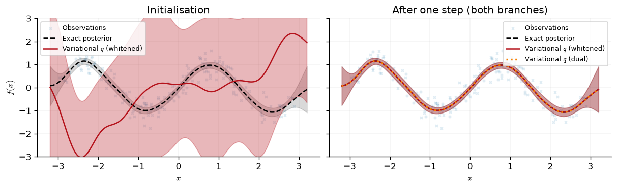
One step from two completely different starting points and two completely different storage conventions — a whitened mean and Cholesky factor on one side, a pair of site parameters on the other — land on the same point to \(3\times10^{-12}\) in the mean and \(3\times10^{-13}\) in the covariance, both measured against the closed-form Titsias optimum, and to \(1\times10^{-13}\) against each other directly. That gap is the float64 noise floor for a problem of this size; both ELBOs agree to the printed six decimal places. This is the cleanest statement this notebook can make about what “two coordinate systems for the same geometry” means: not an analogy, but the same arithmetic answer, reached two different ways.

The plot makes the same point visually — the initial, deliberately absurd \(q\) on the left, and the two stepped posteriors overlaid on the exact GP posterior on the right, indistinguishable from it and from each other.

exact_posterior = unwrapped_regression_model.condition(regression_data)
exact_predictive = exact_posterior(test_inputs)
exact_mean = exact_predictive.mean
exact_stddev = jnp.sqrt(exact_predictive.variance)
whitened_predictive = whitened_stepped(test_inputs)
dual_predictive = dual_stepped(test_inputs)

fig, axes = plt.subplots(ncols=2, figsize=(10, 3.0), sharey=True)
init_predictive = unwrapped_whitened_initial(test_inputs)
for ax, mean_curve, stddev_curve, title in [
    (
        axes[0],
        init_predictive.mean,
        jnp.sqrt(init_predictive.variance),
        "Initialisation",
    ),
    (
        axes[1],
        whitened_predictive.mean,
        jnp.sqrt(whitened_predictive.variance),
        "After one step (both branches)",
    ),
]:
    ax.scatter(
        regression_inputs,
        regression_outputs,
        alpha=0.15,
        s=8,
        color=cols[0],
        label="Observations",
    )
    ax.plot(
        test_inputs, exact_mean, color="black", linestyle="--", label="Exact posterior"
    )
    ax.fill_between(
        test_inputs.flatten(),
        exact_mean - 2 * exact_stddev,
        exact_mean + 2 * exact_stddev,
        alpha=0.15,
        color="black",
    )
    ax.plot(test_inputs, mean_curve, color=cols[1], label="Variational $q$ (whitened)")
    ax.fill_between(
        test_inputs.flatten(),
        mean_curve - 2 * stddev_curve,
        mean_curve + 2 * stddev_curve,
        alpha=0.3,
        color=cols[1],
    )
    ax.set(xlabel=r"$x$", title=title, ylim=(-3.0, 3.0))
axes[1].plot(
    test_inputs,
    dual_predictive.mean,
    color=cols[2],
    linestyle=":",
    linewidth=2,
    label="Variational $q$ (dual)",
)
clean_legend(axes[0])
clean_legend(axes[1])
axes[0].set_ylabel(r"$f(x)$")

Text(0, 0.5, '$f(x)$')

The rest of this notebook is about the second branch: what it stores, where the update in that section came from, and exactly when — not if, when — the two branches stop being the same iteration.

One notational break, from here on. Above, \(\boldsymbol{\theta}\) was the natural parameter of \(q(\mathbf{u})\) and \(\boldsymbol{\eta}\) was the expectation parameter. From here \(\boldsymbol{\theta}\) is reserved for the kernel hyperparameters, which enter for the first time in the hyperparameter-learning section near the end. The natural parameter of \(q(\mathbf{u})\) becomes \(\boldsymbol{\eta}\), the expectation parameter becomes \(\boldsymbol{\mu}\), and \(\boldsymbol{\lambda}\) is the site — not the fixed conjugate-likelihood vector of the derivation just above, which will not be needed again. In these letters the Fisher identity reads \(\tilde\nabla_{\boldsymbol{\eta}}\mathcal{L} = \partial\mathcal{L}/\partial\boldsymbol{\mu}\), and it is restated that way below.

From natural to dual coordinates

Write the natural parameter of \(q(\mathbf{u}) = \mathcal{N}(\mathbf{m},\mathbf{S})\) as \(\boldsymbol{\eta} = (\mathbf{S}^{-1}\mathbf{m},\ -\tfrac12\mathbf{S}^{-1})\), and the natural parameter of the prior \(p(\mathbf{u}) = \mathcal{N}(\mathbf{0},\mathbf{K}_{zz})\) as \(\boldsymbol{\eta}_0(\boldsymbol{\theta}) = (\mathbf{0},\ -\tfrac12\mathbf{K}_{zz}^{-1})\). Their difference is the object this half of the notebook stores:

\[\boldsymbol{\eta} = \underbrace{\left(\mathbf{0},\ -\tfrac12\mathbf{K}_{zz}^{-1}\right)}_{\boldsymbol{\eta}_0(\boldsymbol{\theta})\ \text{prior}} \;+\; \underbrace{\left(\boldsymbol{\lambda}_1,\ -\tfrac12\boldsymbol{\Lambda}_2\right)}_{\boldsymbol{\lambda}\ \text{sites}} .\]

The decomposition is additive, and — in this convention — the second half carries no dependence on the kernel hyperparameters \(\boldsymbol{\theta}\) at all. Equivalently, \(q\) is the prior reweighted by an unnormalised Gaussian site,

\[t(\tilde{\mathbf{u}}) = \exp\!\left(\boldsymbol{\lambda}_1^\top\tilde{\mathbf{u}} - \tfrac12\tilde{\mathbf{u}}^\top\boldsymbol{\Lambda}_2\tilde{\mathbf{u}}\right), \qquad q(\mathbf{u}) \propto p_{\boldsymbol{\theta}}(\mathbf{u})\,t(\tilde{\mathbf{u}}),\]

from which the moments follow by completing the square,

\[\mathbf{S} = \left(\mathbf{K}_{zz}^{-1} + \boldsymbol{\Lambda}_2\right)^{-1}, \qquad \tilde{\mathbf{m}} = \mathbf{S}\boldsymbol{\lambda}_1, \qquad \mathbf{m} = \boldsymbol{\mu}_z + \tilde{\mathbf{m}} .\]

Here \(\tilde{\mathbf{u}} = \mathbf{u} - \boldsymbol{\mu}_z\) are the inducing outputs centred on the prior mean function — exactly the \(\boldsymbol{\mu}_z\) that made the shared demo above need a non-zero mean function to be a fair test. DualVariationalGaussian stores \(\boldsymbol{\lambda}_1\) as dual_vector (\(M\times1\)) and \(\boldsymbol{\Lambda}_2\) as dual_matrix (\(M\times M\)), both defaulting to zero, which sets \(q=p\) and makes the KL vanish at initialisation.

Nothing here is ever inverted. Every quantity the family needs routes through

\[\mathbf{R} := \mathbf{K}_{zz} + \mathbf{K}_{zz}\boldsymbol{\Lambda}_2\mathbf{K}_{zz} = \mathbf{K}_{zz}\mathbf{S}^{-1}\mathbf{K}_{zz},\]

which satisfies \(\mathbf{R} \succeq \mathbf{K}_{zz} \succ 0\) whenever \(\boldsymbol{\Lambda}_2 \succeq 0\). So \(\operatorname{chol}(\mathbf{R})\) cannot fail, and it is better conditioned than \(\operatorname{chol}(\boldsymbol{\Lambda}_2)\) would be, which is rank deficient at initialisation and whenever the batch is smaller than \(M\). Two Cholesky factorisations per iteration, \(\mathbf{L}_K\) and \(\mathbf{L}_R\), and no more.

The EP connection

Where do \(\boldsymbol{\lambda}_1\) and \(\boldsymbol{\Lambda}_2\) come from? Adam et al. [2021] show that the ELBO-optimal \(q\) has the site form

\[q^*(\mathbf{u}) \;\propto\; p_{\boldsymbol{\theta}}(\mathbf{u})\prod_{i=1}^{N} t_i^*(\mathbf{u}), \qquad t_i^*(\mathbf{u}) = \exp\!\left(\langle\boldsymbol{\lambda}_i^*,\ \mathbf{T}(\mathbf{a}_i^\top\mathbf{u})\rangle\right),\]

with \(\mathbf{T}(v) = (v, v^2)\) the Gaussian sufficient statistics and \(\mathbf{a}_i = \mathbf{K}_{zz}^{-1}\mathbf{k}_z(x_i)\). Each \(t_i\) is a two-dimensional object acting on the scalar projection \(\mathbf{a}_i^\top\mathbf{u}\): one local likelihood approximation per data point, exactly as in expectation propagation. The difference from EP is where the site values come from. EP computes them by matching moments against a cavity distribution; here they are read straight off the first two derivatives of the expected log likelihood. With \(q(f_i) = \mathcal{N}(m_i, v_i)\), Bonnet’s and Price’s theorems give

\[\alpha_i = \frac{\partial}{\partial m_i}\,\mathbb{E}_{q(f_i)}\!\left[\log p(y_i\mid f_i)\right], \qquad \beta_i = -2\,\frac{\partial}{\partial v_i}\,\mathbb{E}_{q(f_i)}\!\left[\log p(y_i\mid f_i)\right],\]

so a single jax.grad of the likelihood’s existing expected_log_likelihood suffices. No second derivatives, and it works for closed-form and quadrature likelihoods alike. For a Gaussian likelihood \(\alpha_i = (y_i - m_i)/\sigma^2\) and \(\beta_i = 1/\sigma^2\); here are both, by autodiff.

key, alpha_beta_key = jr.split(key)
ep_response = jr.normal(alpha_beta_key, (5, 1))
ep_mean = jnp.linspace(-1.0, 1.0, 5)
ep_variance = jnp.linspace(0.2, 0.9, 5)
ep_stddev = 0.37
ep_likelihood = gpx.likelihoods.Gaussian(obs_stddev=ep_stddev)


def total_expected_log_likelihood(mean, variance):
    """Summed variational expectation, as a function of the marginal moments."""
    return jnp.sum(
        ep_likelihood.expected_log_likelihood(
            ep_response, mean[:, None], variance[:, None]
        )
    )


bonnet_alpha, price_derivative = jax.grad(
    total_expected_log_likelihood, argnums=(0, 1)
)(ep_mean, ep_variance)
price_beta = -2.0 * price_derivative

closed_form_alpha = (ep_response.squeeze(-1) - ep_mean) / ep_stddev**2
closed_form_beta = jnp.full_like(ep_mean, 1.0 / ep_stddev**2)

print(
    "max |alpha - (y - m) / sigma^2| : "
    f"{jnp.max(jnp.abs(bonnet_alpha - closed_form_alpha)):.3e}"
)
print(
    "max |beta - 1 / sigma^2|        : "
    f"{jnp.max(jnp.abs(price_beta - closed_form_beta)):.3e}"
)
print(f"beta                            : {price_beta[0]:.6f} (= 1 / {ep_stddev}^2)")

max |alpha - (y - m) / sigma^2| : 8.882e-15
max |beta - 1 / sigma^2|        : 4.441e-15
beta                            : 7.304602 (= 1 / 0.37^2)

Both match the closed form to \(10^{-14}\). Stored naively that is \(\mathcal{O}(N)\) memory, which would be a poor trade. But every \(t_i\) enters \(q(\mathbf{u})\) only through the rank-one projection \(\mathbf{a}_i^\top\mathbf{u}\), so the \(N\) sites can be tied: summed into two inducing-space objects of size \(M\) and \(M\times M\). Writing \(g_{1,i} = \alpha_i + \beta_i\,(m_i - \mu(x_i))\) and \(g_{2,i} = \beta_i\), the tied values at a converged full-batch E-step are

\[\boldsymbol{\lambda}_1 = \sum_{i=1}^{N}\mathbf{a}_i g_{1,i} = \mathbf{A}\mathbf{g}_1, \qquad \boldsymbol{\Lambda}_2 = \sum_{i=1}^{N}g_{2,i}\,\mathbf{a}_i\mathbf{a}_i^\top = \mathbf{A}\operatorname{diag}(\mathbf{g}_2)\mathbf{A}^\top .\]

Memory is back to \(\mathcal{O}(M^2)\), the same as standard SVGP. Two warnings. The tying introduces a bias — the paper says so, and reports that it “does not seem to affect convergence in practice.” And these sums are the fixed point, not the value at a general iterate: during training the stored pair is a running convex combination of such targets, and is never computed by evaluating the sum.

Two silent convention traps

Two traps wait for anyone reading the paper alongside the code, and both are silent: each produces a valid-looking \(q\) that is simply not the one intended.

The flanking trap. The paper’s main text stores the un-flanked sums, built from \(\mathbf{k}_z(x_i)\) rather than \(\mathbf{a}_i = \mathbf{K}_{zz}^{-1}\mathbf{k}_z(x_i)\): \(\bar{\boldsymbol{\lambda}}_1 = \mathbf{K}_{zz}\boldsymbol{\lambda}_1\), \(\bar{\boldsymbol{\Lambda}}_2 = \mathbf{K}_{zz}\boldsymbol{\Lambda}_2\mathbf{K}_{zz}\). Both conventions describe the same \(q\) and give the same \(\mathbf{R}\), but they are not interchangeable for our purposes: the additive, hyperparameter-free split of the previous section holds exactly only in the flanked convention, since in the un-flanked one \(\boldsymbol{\eta}_1 = \mathbf{K}_{zz}^{-1}\bar{\boldsymbol{\lambda}}_1\) moves with \(\boldsymbol{\theta}\) too. The paper flags the choice in a single sentence and calls the flanked form “an alternative tying method”; GPJax stores the alternative.

The \(-\tfrac12\) trap. The paper uses \(\lambda_2\) with two incompatible meanings across its own equations: a natural-parameter one (\(-\tfrac12\beta_i\)) and a precision one (\(g_{2,i} = \beta_i\)). The dense limit settles it — with \(\mathbf{Z}=\mathbf{X}\), \(\mathbf{S}^{-1} = \mathbf{K}_{ff}^{-1} + \operatorname{diag}(\boldsymbol{\beta})\) forces \(\boldsymbol{\Lambda}_2 = \operatorname{diag}(\boldsymbol{\beta})\), positive. GPJax stores \(\boldsymbol{\Lambda}_2\) in the precision convention: positive semi-definite, no \(-\tfrac12\).

The flanked convention is not free: storing \(\boldsymbol{\Lambda}_2\) rather than \(\bar{\boldsymbol{\Lambda}}_2\) means a round trip through \(\mathbf{K}_{zz}^{-1}\) and back, which squares its condition number. That is dramatic entrywise, invisible in everything anyone actually reads off the model, and cheap to measure. Put the inducing inputs on the data themselves, \(\mathbf{Z}=\mathbf{X}\), for the first forty points of the conjugate regression above — the worst case for \(\operatorname{cond}(\mathbf{K}_{zz})\), and the one configuration in which the optimal sites are known on paper: \(\boldsymbol{\lambda}_1 = (\mathbf{y}-\boldsymbol{\mu}_x)/\sigma^2\) and \(\boldsymbol{\Lambda}_2 = \mathbf{I}/\sigma^2\). One \(\rho=1\) step lands on that fixed point, exactly as in the shared demo, and what the family then stores can be compared entrywise against the paper answer.

dense_count = 40
dense_inputs = regression_inputs[:dense_count]
dense_data = gpx.Dataset(X=dense_inputs, y=regression_outputs[:dense_count])

dense_variational, dense_hyper = partition_variational(
    DualVariationalGaussian(model=regression_model, inducing_inputs=dense_inputs)
)
dense_variational, _ = natural_gradient_step(
    dense_variational, dense_hyper, dense_data, negative_dual_elbo, 1.0
)
dense_fitted = paramax.unwrap(eqx.combine(dense_variational, dense_hyper))

dense_gram = regression_kernel.gram(dense_inputs).as_matrix() + (
    regression_jitter * jnp.eye(dense_count)
)
dense_centred = dense_data.y - regression_mean_function(dense_inputs)
exact_dual_vector = dense_centred / observation_variance
exact_dual_matrix = jnp.eye(dense_count) / observation_variance
flanked_error = jnp.max(
    jnp.abs(dense_gram @ (dense_fitted.dual_vector - exact_dual_vector))
)
flanked_scale = jnp.max(jnp.abs(dense_gram @ exact_dual_vector))

print(f"cond(K_zz) at Z = X             : {jnp.linalg.cond(dense_gram):.3e}")
print(
    "max |Lambda_2 - I / sigma^2|    : "
    f"{jnp.max(jnp.abs(dense_fitted.dual_matrix - exact_dual_matrix)):.3e}"
    "   (never test this)"
)
print(
    "relative error of K_zz lambda_1 : "
    f"{float(flanked_error / flanked_scale):.3e}   (test this instead)"
)

cond(K_zz) at Z = X             : 1.042e+09
max |Lambda_2 - I / sigma^2|    : 8.384e+00   (never test this)
relative error of K_zz lambda_1 : 2.590e-09   (test this instead)

The stored matrix is wrong by \(8.4\) entrywise — against an analytic answer whose every diagonal entry is \(1/\sigma^2 \approx 11.1\) — because forming it routes through \(\mathbf{K}_{zz}^{-1}\) at a condition number of \(10^{9}\). Yet the flanked quantity \(\mathbf{K}_{zz}\boldsymbol{\lambda}_1\), which is what everything downstream actually consumes, is right to \(2.6\times10^{-9}\) in relative error: the error lives in the near-null space of \(\mathbf{K}_{zz}\) and is annihilated on the way back out. A measurement in one configuration, not a theorem — and the rule it teaches is the one to keep: GPJax stores the flanked, precision convention; never test \(\boldsymbol{\Lambda}_2\) entrywise — test \(\mathbf{R}\), the moments, or the predictions instead.

The tied natural-gradient update

Now the payoff. Split the ELBO into its two terms, with \(\boldsymbol{\mu}\) the expectation parameter of \(q\):

\[\mathcal{L}(\boldsymbol{\eta}) = \mathcal{L}_{\text{ell}}(\boldsymbol{\eta}) - \operatorname{KL}\left[q_{\boldsymbol{\eta}}\,\|\,p_{\boldsymbol{\eta}_0}\right], \qquad \mathcal{L}_{\text{ell}} = \frac{N}{B}\sum_{i\in\mathcal{B}}\mathbb{E}_{q(f_i)}\!\left[\log p(y_i\mid f_i)\right].\]

For an exponential family the KL between two of its members is \(\langle\boldsymbol{\eta}-\boldsymbol{\eta}_0,\boldsymbol{\mu}\rangle - A(\boldsymbol{\eta}) + A(\boldsymbol{\eta}_0)\), and \(\nabla_{\boldsymbol{\eta}}A = \boldsymbol{\mu}\), so the two Jacobian terms cancel and

\[\nabla_{\boldsymbol{\mu}}\operatorname{KL}\left[q_{\boldsymbol{\eta}}\,\|\,p_{\boldsymbol{\eta}_0}\right] = \boldsymbol{\eta} - \boldsymbol{\eta}_0 = \boldsymbol{\lambda} .\]

The KL’s gradient is the stored parameter itself. Since the natural gradient in \(\boldsymbol{\eta}\) is the ordinary gradient in \(\boldsymbol{\mu}\) — the Fisher identity from the first half of this notebook, restated in the new letters — the ascent step \(\boldsymbol{\eta} \leftarrow \boldsymbol{\eta} + \rho\,\nabla_{\boldsymbol{\mu}}\mathcal{L}\) collapses to

\[\boldsymbol{\lambda} \;\leftarrow\; (1-\rho)\,\boldsymbol{\lambda} \;+\; \rho\,\nabla_{\boldsymbol{\mu}}\mathcal{L}_{\text{ell}},\]

a convex combination between where the sites are and where this mini-batch wants them. The KL never has to be differentiated at all. Chaining \(\nabla_{\boldsymbol{\mu}}\mathcal{L}_{\text{ell}}\) through the marginals and converting out of the \(-\tfrac12\) convention gives the update in stored coordinates,

\[\boldsymbol{\lambda}_1 \leftarrow (1-\rho)\boldsymbol{\lambda}_1 + \rho\,\frac{N}{B}\,\mathbf{A}_{\mathcal{B}}\mathbf{g}_1^{\mathcal{B}}, \qquad \boldsymbol{\Lambda}_2 \leftarrow (1-\rho)\boldsymbol{\Lambda}_2 + \rho\,\frac{N}{B}\,\mathbf{A}_{\mathcal{B}}\operatorname{diag}\!\left(\mathbf{g}_2^{\mathcal{B}}\right)\mathbf{A}_{\mathcal{B}}^\top .\]

The \(N/B\) factor is not in the paper’s printed update; without it the sites converge to \(B/N\) of their correct value, since a mini-batch sum is \(B/N\) of the full sum in expectation. GPJax supplies it.

Two consequences worth stating separately. First, the update is affine in the stored parameters, so for \(\rho\in[0,1]\) and \(\beta_i\ge0\) it can never leave the positive semi-definite cone: a convex combination of PSD matrices is PSD. Second, \(\rho\) is the Salimbeni step size \(\gamma\) from the first half of this notebook, not a separate damping coefficient — the display above is \(\boldsymbol{\eta}\leftarrow\boldsymbol{\eta}+\rho\nabla_{\boldsymbol{\mu}}\mathcal{L}\) written out. GPJax accordingly uses one keyword, natgrad_lr, for both dispatch branches; the shared conjugate demo two sections back already used 1.0 for both. The cone-safety section below checks the two branches against each other step by step at \(\rho=\gamma=0.8\).

It is worth being concrete about what the site step does not do. A natural-gradient step in the moment parameterisation \((\mathbf{m},\mathbf{L})\) has to convert to \(\boldsymbol{\eta}\), differentiate the whole ELBO — Cholesky of \(\mathbf{K}_{zz}\), the conditional, and the KL — apply a Jacobian, and then convert back through \(\boldsymbol{\theta}\), which costs an inverse and a fresh Cholesky. In site coordinates none of that happens, for two structural reasons: the stored coordinates are an affine image of \(\boldsymbol{\eta}\), so the step is an affine step on them directly; and the target \(\nabla_{\boldsymbol{\mu}}\mathcal{L}_{\text{ell}}\) has a closed form whose only dependence on \(q\) is through the marginals \((m_i, v_i)\), which the ELBO computes anyway.

stage	site (dual)	natural gradients on \((\mathbf{m},\mathbf{L})\)
\(\operatorname{chol}(\mathbf{K}_{zz})\)	\(\mathcal{O}(M^3)\)	\(\mathcal{O}(M^3)\)
\(\mathbf{A}_{\mathcal{B}} = \mathbf{K}_{zz}^{-1}\mathbf{K}_{zb}\)	\(\mathcal{O}(M^2B)\)	\(\mathcal{O}(M^2B)\)
covariance factor	\(\operatorname{chol}(\mathbf{R})\), \(\mathcal{O}(M^3)\)	\(\mathbf{S} = \mathbf{L}\mathbf{L}^\top\), \(\mathcal{O}(M^3)\)
marginals \((m_i, v_i)\)	\(\mathcal{O}(M^2B)\)	\(\mathcal{O}(M^2B)\)
\((\boldsymbol{\alpha},\boldsymbol{\beta})\)	one jax.grad of a scalar in two \(B\)-vectors	the same, but inside the full AD tape
gradient assembly	two einsums, \(\mathcal{O}(M^2B)\)	reverse-mode AD through chol / conditional / KL, plus a Jacobian
\(\boldsymbol{\eta}\to\boldsymbol{\xi}\) round trip	none	inverse + Cholesky, \(\mathcal{O}(M^3)\)

Same asymptotics, with strictly less work on the site side of the table. Whether that turns into wall-clock depends on how large a share of the iteration the saved work was; the dual sparse GP notebook measures it on a real training run. What is certain is the direction of any difference: since the iterates are the same either way (subject to the cone-safety condition below), the E-step can only differ in time, never in accuracy. Adam et al. measure about \(5\times\) on MNIST (\(N = 70{,}000\), \(M = 100\), \(B = 200\), ten latent GPs) against GPflow’s SVGP with natural gradients, with the caveat that their “implementation is not as optimized as SVGP in GPflow.”

Cone-safety

The step is \(\boldsymbol{\theta}\leftarrow\boldsymbol{\theta} - \gamma\,\partial\ell/\partial\boldsymbol{\eta}\) (moment coordinates) or \(\boldsymbol{\lambda} \leftarrow (1-\rho)\boldsymbol{\lambda} + \rho\,\nabla_{\boldsymbol{\mu}}\mathcal{L}_{\text{ell}}\) (site coordinates), and each has a cone it must not leave: \(\boldsymbol{\Theta}_2 \prec 0\) because it is \(-\tfrac12\) a covariance inverse, and \(\boldsymbol{\Lambda}_2 \succeq 0\) because it is a precision. Nothing in either update enforces that automatically. We take the two cones in turn.

Moment coordinates: the negative-definite cone. Splitting the ELBO as \(\mathcal{L} = \mathcal{L}_{\text{data}} - \operatorname{KL}[q\,\|\,p]\) and using \(\partial\operatorname{KL}/\partial\mathbf{S} = \tfrac12\mathbf{K}_{zz}^{-1} - \tfrac12\mathbf{S}^{-1}\) gives an exact description of the step:

\[\boldsymbol{\Theta}_2^{\text{new}} = (1-\gamma)\,\boldsymbol{\Theta}_2 + \gamma\,\boldsymbol{\Theta}_2^{\text{tgt}}, \qquad \boldsymbol{\Theta}_2^{\text{tgt}} := \frac{\partial\mathcal{L}_{\text{data}}}{\partial\mathbf{S}} - \tfrac{1}{2}\mathbf{K}_{zz}^{-1}\]

(for the whitened family, replace \(\mathbf{K}_{zz}^{-1}\) by \(\mathbf{I}_M\)). So the step is a convex combination in \(\boldsymbol{\theta}\)-space whenever \(\gamma\in[0,1]\) — the mirror-descent reading, made concrete.

Cone-safety theorem (moments). If the likelihood is log-concave in \(f\), then by Price’s theorem (\(\partial_{\mathbf{S}}\mathbb{E}_{\mathcal{N}(\mathbf{m},\mathbf{S})}[g] = \tfrac12\mathbb{E}[\nabla^2 g]\)),

\[\frac{\partial\mathcal{L}_{\text{data}}}{\partial\mathbf{S}} = \frac{N}{B}\sum_{n\in\mathcal{B}}\tfrac{1}{2}\,\mathbb{E}_{q(f_n)}\!\left[\frac{\partial^2\log p(y_n\mid f_n)}{\partial f_n^2}\right]\mathbf{a}_n\mathbf{a}_n^\top \preceq 0,\]

where \(\mathbf{a}_n^\top\) is row \(n\) of \(\mathbf{A} = \mathbf{K}_{xz}\mathbf{K}_{zz}^{-1}\). Hence \(\boldsymbol{\Theta}_2^{\text{tgt}} \prec 0\), and for \(\gamma\in[0,1]\) \(\boldsymbol{\Theta}_2^{\text{new}}\) is a convex combination of two negative-definite matrices, so it is negative definite. Mini-batching does not break this, because \(N/B>0\) preserves the sign. \(\square\)

Two things escape the theorem: \(\gamma>1\), which extrapolates past \(\boldsymbol{\Theta}_2^{\text{tgt}}\); and likelihoods that are not log-concave as computed — GPJax’s inv_probit clips its output into \([10^{-3},1-10^{-3}]\), which flattens \(\log p\) enough to give it a positive second derivative for \(f\lesssim-2.44\), so even the Bernoulli model below leaves the guaranteed regime once a point is confidently mislabelled. We sweep \(\gamma\) from an over-confident starting point, \(\mathbf{S}_0=10^{-2}\mathbf{I}\), sharper than the target — precisely the regime where extrapolation bites — on the two-dimensional “banana” classification problem used again below.

def make_banana(key, num_points):
    """Two-class banana problem with a curved Bayes-optimal boundary."""
    key_latent, key_label = jr.split(key)
    latent = jr.uniform(key_latent, (num_points, 2), minval=-3.0, maxval=3.0)
    decision = latent[:, 1] - (0.7 * latent[:, 0] ** 2 - 1.5)
    probability = jax.nn.sigmoid(3.0 * decision)
    labels = (jr.uniform(key_label, (num_points,)) < probability).astype(jnp.float64)
    return latent, labels[:, None]


banana_key = jr.key(42)
banana_inputs, banana_labels = make_banana(banana_key, 2000)
num_train = 1600
banana_train = gpx.Dataset(X=banana_inputs[:num_train], y=banana_labels[:num_train])

num_banana_inducing = 50
inducing_grid = jnp.meshgrid(jnp.linspace(-2.8, 2.8, 10), jnp.linspace(-2.8, 2.8, 5))
banana_inducing = jnp.stack([axis.ravel() for axis in inducing_grid], axis=1)

banana_model = (
    gpx.gps.Prior(
        mean_function=gpx.mean_functions.Zero(), kernel=jk.RBF(active_dims=[0, 1])
    )
    * gpx.likelihoods.Bernoulli()
)

overconfident_family = VariationalGaussian(
    model=banana_model,
    inducing_inputs=banana_inducing,
    variational_mean=jnp.zeros((num_banana_inducing, 1)),
    variational_root_covariance=0.1 * jnp.eye(num_banana_inducing),
)
overconfident_mean = overconfident_family.variational_mean.unwrap()
overconfident_root = overconfident_family.variational_root_covariance.unwrap()


def banana_loss_of_expectation(expectation):
    variational_mean, variational_root = moments_from_expectation(*expectation)
    trial = eqx.tree_at(
        lambda family: (family.variational_mean, family.variational_root_covariance),
        overconfident_family,
        (Real(variational_mean), LowerTriangular(variational_root)),
    )
    return negative_elbo(paramax.unwrap(trial), banana_train)


cone_gradient = jax.grad(banana_loss_of_expectation)(
    expectation_from_moments(overconfident_mean, overconfident_root)
)
# The matrix statistic is symmetric, so symmetrise the entrywise autodiff gradient.
matrix_gradient = 0.5 * (cone_gradient[1] + cone_gradient[1].T)
_, natural_matrix = natural_from_moments(overconfident_mean, overconfident_root)

gamma_values = jnp.array([0.1, 0.5, 1.0, 2.0, 5.0, 10.0])
largest_eigenvalues = jnp.array(
    [
        jnp.max(jnp.linalg.eigvalsh(natural_matrix - g * matrix_gradient))
        for g in gamma_values
    ]
)
print("gamma      max eig(Theta2_new)   status")
for gamma, largest in zip(gamma_values, largest_eigenvalues, strict=True):
    status = "negative definite" if largest < 0 else "*** LEFT THE CONE ***"
    print(f"{float(gamma):6.2f}   {float(largest):+18.5f}   {status}")

fig, ax = plt.subplots(figsize=(5.5, 3.2))
ax.plot(gamma_values, largest_eigenvalues, marker="o", color=cols[1])
ax.axhline(0.0, color="black", linestyle="--", linewidth=1)
ax.axvline(1.0, color="gray", linestyle=":", linewidth=1)
ax.set(
    xlabel=r"$\gamma$",
    ylabel=r"$\lambda_{\max}(\boldsymbol{\Theta}_2^{\text{new}})$",
    title="Where this initialisation leaves the cone",
)

gamma      max eig(Theta2_new)   status
  0.10            -45.46684   negative definite
  0.50            -27.33418   negative definite
  1.00             -4.66836   negative definite
  2.00            +40.66328   *** LEFT THE CONE ***
  5.00           +176.65821   *** LEFT THE CONE ***
 10.00           +403.31642   *** LEFT THE CONE ***

[Text(0.5, 0, '$\\gamma$'),
 Text(0, 0.5, '$\\lambda_{\\max}(\\boldsymbol{\\Theta}_2^{\\text{new}})$'),
 Text(0.5, 1.0, 'Where this initialisation leaves the cone')]

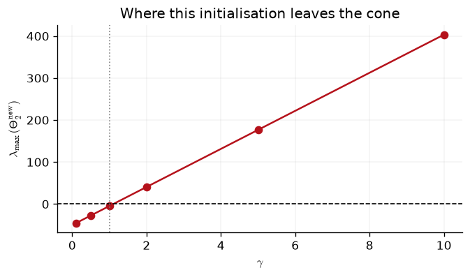
Read that as a statement about this initialisation, not about \(\gamma=2\) in general. Here \(\mathbf{S}_0=10^{-2}\mathbf{I}\) makes \(\boldsymbol{\Theta}_2=-50\mathbf{I}\), an order of magnitude sharper than the target, so the convex combination has little room to extrapolate into: the sign flips between \(\gamma=1\) (\(-4.67\)) and \(\gamma=2\) (\(+40.66\)), and linear interpolation puts the crossing at \(\gamma\approx1.10\). What the theorem actually guarantees is \(\gamma\in[0,1]\), for any log-concave likelihood and any starting point, and nothing whatsoever beyond that.

When it does go wrong, jnp.linalg.cholesky returns NaN rather than raising, which means validity is a value and the fix stays jit-compatible: natural_gradient_step evaluates the trial steps \(\{\gamma\beta^k\}_{k=0}^{K}\) under vmap and selects the first one whose Cholesky is finite. backoff (\(\beta\), default \(0.5\)) and max_backoff (\(K\), default \(5\)) are exposed by fit_natgrads. This backoff is specific to the moment branch — the site branch’s affine update needs no such rescue, for the reason the rest of this section develops.

Site coordinates: the positive-semidefinite cone. The tied update derived above is affine in \(\boldsymbol{\lambda}\), so for \(\rho\in[0,1]\) a convex combination of \(\boldsymbol{\Lambda}_2\succeq0\) and a PSD target stays PSD automatically — no Cholesky-validity check is needed, because there is nothing to fail. The one place this can still go wrong is upstream of the convex combination: the target itself is built from Price’s curvature \(\beta_i\), and \(\beta_i\ge0\) needs the same log-concavity condition as the moment branch’s cone-safety theorem — as computed, not as written. GPJax’s dual step guards this with a floor, beta_floor (default \(10^{-8}\)), clipping \(\boldsymbol{\beta}\) from below before it enters \(\boldsymbol{\Lambda}_2\). It is \(\boldsymbol{\beta}\) that is clipped, never \(\boldsymbol{\Lambda}_2\) itself, so the update stays affine and jit/scan-safe.

Since \(\rho=\gamma\), the two branches should step identically — the same \((\mathbf{m},\mathbf{S})\) at every iteration — for as long as the computed \(\beta_i\) stay non-negative, and only then. We check this directly: six matched \(\rho=\gamma=0.8\) steps on the banana problem, both branches started at \(q=p\), comparing \((\mathbf{m},\mathbf{S})\) after every step and recording Price’s curvature just before it.

def implied_moments(family):
    """Return $(m, S)$ for either parameterisation."""
    unwrapped = paramax.unwrap(family)
    if isinstance(unwrapped, DualVariationalGaussian):
        return unwrapped.moments()
    root = unwrapped.variational_root_covariance
    return unwrapped.variational_mean, root @ root.T


def make_banana_moment_family():
    """A fresh SVGP over the banana data, at q = p."""
    banana_gram = paramax.unwrap(banana_model).prior.kernel.gram(
        banana_inducing
    ).as_matrix() + 1e-6 * jnp.eye(num_banana_inducing)
    return VariationalGaussian(
        model=banana_model,
        inducing_inputs=banana_inducing,
        variational_mean=jnp.zeros((num_banana_inducing, 1)),
        variational_root_covariance=jnp.linalg.cholesky(banana_gram),
    )


def price_curvature(family, data):
    """Return the marginal means and $\\beta_i=-2\\,\\partial_{v_i}E_q[\\log p]$."""
    marginal_mean, marginal_variance = family.marginals(data.X)

    def total_expectation(variance):
        return jnp.sum(
            family.model.likelihood.expected_log_likelihood(
                data.y, marginal_mean[:, None], variance[:, None]
            )
        )

    return marginal_mean, -2.0 * jax.grad(total_expectation)(marginal_variance)


def six_matched_steps(beta_floor):
    """Six rho = 0.8 steps in both branches, from the shared q = p start."""
    site_partition, site_hyper = partition_variational(
        DualVariationalGaussian(model=banana_model, inducing_inputs=banana_inducing)
    )
    moment_partition, moment_hyper = partition_variational(make_banana_moment_family())
    rows = []
    for _ in range(6):
        # Measured before the step, at the q both branches currently share.
        marginal_mean, curvature = price_curvature(
            paramax.unwrap(eqx.combine(site_partition, site_hyper)), banana_train
        )
        site_partition, _ = natural_gradient_step(
            site_partition,
            site_hyper,
            banana_train,
            negative_dual_elbo,
            0.8,
            beta_floor=beta_floor,
        )
        moment_partition, _ = natural_gradient_step(
            moment_partition, moment_hyper, banana_train, negative_elbo, 0.8
        )
        site_mean, site_covariance = implied_moments(
            eqx.combine(site_partition, site_hyper)
        )
        moment_mean, moment_covariance = implied_moments(
            eqx.combine(moment_partition, moment_hyper)
        )
        rows.append(
            (
                max(
                    float(jnp.max(jnp.abs(site_mean - moment_mean))),
                    float(jnp.max(jnp.abs(site_covariance - moment_covariance))),
                ),
                int(jnp.sum(curvature < 0)),
                float(jnp.min(curvature)),
                float(marginal_mean[jnp.argmin(curvature)]),
            )
        )
    return rows


floored_rows = six_matched_steps(1e-8)
print("step   |(m, S) gap|   beta < 0   min beta   its marginal mean")
for step, (gap, negative_count, smallest, mean_there) in enumerate(
    floored_rows, start=1
):
    print(
        f"{step:4d}   {gap:12.3e}   {negative_count:4d}/{banana_train.n}"
        f"   {smallest:+8.4f}   {mean_there:+8.3f}"
    )

banana_gap = max(gap for gap, _, _, _ in floored_rows)
unfloored_rows = six_matched_steps(-jnp.inf)
unfloored_gap = max(gap for gap, _, _, _ in unfloored_rows)
print(f"\nworst gap, default beta_floor = 1e-8 : {banana_gap:.3e}")
print(f"worst gap, clip disabled (-inf)      : {unfloored_gap:.3e}")

fig, ax = plt.subplots(figsize=(5.5, 3.2))
steps = jnp.arange(1, 7)
ax.plot(
    steps,
    jnp.array([g for g, _, _, _ in floored_rows]),
    marker="o",
    color=cols[1],
    label="default beta_floor",
)
ax.plot(
    steps,
    jnp.array([g for g, _, _, _ in unfloored_rows]),
    marker="x",
    color=cols[0],
    label="clip disabled",
)
ax.set(
    xlabel="Step",
    ylabel=r"$\max|(\mathbf{m}, \mathbf{S})_{\text{site}} - (\mathbf{m}, \mathbf{S})_{\text{moment}}|$",
    yscale="log",
    title="The two branches, step by step",
)
clean_legend(ax)

step   |(m, S) gap|   beta < 0   min beta   its marginal mean
   1      9.770e-14      0/1600    +0.5622     +0.000
   2      7.860e-14      0/1600    +0.1454     +1.889
   3      1.288e-13      0/1600    +0.0725     +2.347
   4      1.479e-13      0/1600    +0.0369     -2.669
   5      1.717e-03      1/1600    -0.2626     +2.427
   6      5.104e-03      1/1600    -0.4955     +2.521

worst gap, default beta_floor = 1e-8 : 5.104e-03
worst gap, clip disabled (-inf)      : 3.748e-13

<Axes: title={'center': 'The two branches, step by step'}, xlabel='Step', ylabel='$\\max|(\\mathbf{m}, \\mathbf{S})_{\\text{site}} - (\\mathbf{m}, \\mathbf{S})_{\\text{moment}}|$'>

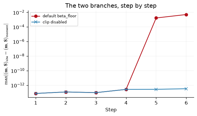
For the first four steps every \(\beta_i\) is positive, the clip does nothing, and the two branches agree to \(\sim10^{-13}\) — the float64 noise floor. At step five a single training point out of 1600 crosses into \(\beta_i<0\) — a label-\(0\) point, whose log-likelihood is the \(f\mapsto-f\) mirror of the \(y=1\) case, so the \(-2.44\) threshold derived above sits at \(+2.44\) for it, and its marginal mean has just reached \(+2.427\) — the beta_floor clip engages, and from that step the gap jumps to \(\mathcal{O}(10^{-3})\) and compounds at step six. Disabling the clip (beta_floor=-jnp.inf, the second line above) brings the same six steps back to the noise floor — \(8.9\times10^{-13}\) — which pins the cause down precisely: it is neither conditioning nor the cancellation in \(\mathbf{H}_2=\mathbf{S}+\mathbf{m}\mathbf{m}^\top\) that the moment branch has to undo, since disabling the one thing that differs between the branches removes the discrepancy entirely. The condition the \(\rho=\gamma\) identity needs — \(\beta_i\ge0\), log-concavity as computed — is real, and this is exactly where and how it fails, on the same problem and the same clip that guarantees the site branch never leaves its own cone. The residual is still far below anything visible in the ELBO, which is the number either optimiser is steering by.

The M-step objective: dual_elbo versus elbo

Variational EM alternates an E-step, which maximises the ELBO over \(q\) at fixed \(\boldsymbol{\theta}\), with an M-step, which maximises it over \(\boldsymbol{\theta}\) at fixed \(q\). “Fixed \(q\)” is the ambiguous part. In natural coordinates the E-step returns \(\boldsymbol{\eta}^*_t = \boldsymbol{\eta}_0(\boldsymbol{\theta}_t) + \boldsymbol{\lambda}^*_t\), and there are two ways to hold that still:

\[\text{standard:}\quad l(\boldsymbol{\theta}) = \mathcal{L}\big(\underbrace{\boldsymbol{\eta}_0(\boldsymbol{\theta}_t) + \boldsymbol{\lambda}^*_t}_{\text{all frozen}},\ \boldsymbol{\theta}\big), \qquad\qquad \text{dual:}\quad \bar l(\boldsymbol{\theta}) = \mathcal{L}\big(\boldsymbol{\eta}_0(\boldsymbol{\theta}) + \boldsymbol{\lambda}^*_t,\ \boldsymbol{\theta}\big).\]

elbo computes the first, because a VariationalGaussian stores \((\mathbf{m},\mathbf{L})\) and those are what stay fixed. dual_elbo computes the second, because a DualVariationalGaussian stores the sites, and the prior half of \(q\) is rebuilt from \(\mathbf{K}_{zz}(\boldsymbol{\theta})\) every time the bound is evaluated. The intuition is that the sites encode what the data said, which is a property of the likelihood and should not be re-derived when the kernel moves, whereas the prior contribution to \(q\) should move with the kernel. That is also why nothing derived from \(\boldsymbol{\theta}\) may be cached on the family — caching \((\mathbf{m},\mathbf{S})\) would turn dual_elbo back into elbo under differentiation while leaving every printed value identical, a silent bug of the worst kind.

Here is what is actually guaranteed, which is less than the headline suggests:

claim	status
\(\bar l\) is a valid lower bound on \(\log p_{\boldsymbol{\theta}}(\mathbf{y})\) everywhere	proven — it is the ELBO at a legitimate Gaussian \(q\)
\(\bar l(\boldsymbol{\theta}_t) = l(\boldsymbol{\theta}_t)\)	proven, exactly, at a converged E-step
\(\nabla_{\boldsymbol{\theta}}\bar l(\boldsymbol{\theta}_t) = \nabla_{\boldsymbol{\theta}}l(\boldsymbol{\theta}_t)\)	proven, same condition, by the envelope theorem
\(\bar l(\boldsymbol{\theta}) \ge l(\boldsymbol{\theta})\) for all \(\boldsymbol{\theta}\)	proven only when the sites are genuinely \(\boldsymbol{\theta}\)-free — a conjugate likelihood with its exact sites and \(\mathbf{Z} = \mathbf{X}\)
\(\bar l\) is a local upper bound on \(l\)	proven in the conjugate case; the paper writes “we can’t show this in the non-conjugate setting”
faster EM convergence when non-conjugate	empirical only — “exact theoretical reasons behind the speed-ups are currently unknown to us”

The first row is free: any Gaussian \(q\), whatever produced it, gives a valid ELBO. The second and third rows are the envelope theorem doing real work — at a stationary \(q\) the implicit dependence of \(\boldsymbol{\eta}_0(\boldsymbol{\theta})\)’s contribution on \(\boldsymbol{\theta}\) contributes nothing to the total derivative, so it does not matter whether the prior half of \(q\) is allowed to move with \(\boldsymbol{\theta}\) or not; away from stationarity it matters a great deal, since nobody runs an E-step to convergence between Adam steps in practice. The fourth and fifth rows need the sites to carry no implicit \(\boldsymbol{\theta}\)-dependence, which is only exactly true without sparsity: with \(\mathbf{Z}\neq\mathbf{X}\) the flanked sites still route through \(\mathbf{K}_{zx}(\boldsymbol{\theta})\), so freezing them at \(\boldsymbol{\theta}_t\) can make \(\bar l\) sub-optimal, and in fact non-dominant, elsewhere. The sixth row is honestly labelled: the paper measures a speed-up and does not derive one.

The claim we can check directly here is rows two and three: value and gradient equality, and how quickly they set in as the E-step converges. Two matched families — sites and moments, started at the same \(q\) — take an increasing number of \(\rho=\gamma=0.8\) E-steps before we read off the hyperparameter gradient of each bound.

num_logit_data = 200
num_logit_inducing = 8
logit_jitter = 1e-8

key, logit_input_key, logit_label_key = jr.split(key, 3)
logit_inputs = jr.uniform(logit_input_key, (num_logit_data, 1), minval=-2.0, maxval=2.0)
logit_labels = (
    jr.uniform(logit_label_key, (num_logit_data, 1))
    < jax.nn.sigmoid(3.0 * jnp.sin(2.0 * logit_inputs))
).astype(jnp.float64)
logit_data = gpx.Dataset(X=logit_inputs, y=logit_labels)
logit_inducing = jnp.linspace(-2.0, 2.0, num_logit_inducing).reshape(-1, 1)

logit_model = (
    gpx.gps.Prior(
        mean_function=gpx.mean_functions.Zero(),
        kernel=jk.RBF(lengthscale=0.5, variance=1.7),
    )
    * gpx.likelihoods.Bernoulli()
)

logit_dual = DualVariationalGaussian(model=logit_model, inducing_inputs=logit_inducing)
logit_gram = paramax.unwrap(logit_model).prior.kernel.gram(
    logit_inducing
).as_matrix() + logit_jitter * jnp.eye(num_logit_inducing)
logit_moments = VariationalGaussian(
    model=logit_model,
    inducing_inputs=logit_inducing,
    variational_mean=jnp.zeros((num_logit_inducing, 1)),
    variational_root_covariance=jnp.linalg.cholesky(logit_gram),
)

shared_bound = float(
    dual_elbo(paramax.unwrap(logit_dual), logit_data)
    - elbo(paramax.unwrap(logit_moments), logit_data)
)
print(f"dual_elbo - elbo at the shared q = p init : {shared_bound:.3e}")


def kernel_gradient(variational, hyper, objective, dataset):
    """Gradient of `objective` with respect to the unconstrained kernel parameters."""

    def loss(hyper):
        return objective(paramax.unwrap(eqx.combine(variational, hyper)), dataset)

    gradient = eqx.filter_grad(loss)(hyper)
    leaves = jtu.tree_leaves(gradient.model.prior.kernel)
    return jnp.concatenate([jnp.atleast_1d(jnp.ravel(leaf)) for leaf in leaves])


print("\nE-steps   max |grad dual_elbo - grad elbo|   |grad dual_elbo|")
for num_e_steps in [0, 1, 3, 6, 20, 60]:
    site_partition, site_hyper = partition_variational(logit_dual)
    moment_partition, moment_hyper = partition_variational(logit_moments)
    for _ in range(num_e_steps):
        site_partition, _ = natural_gradient_step(
            site_partition, site_hyper, logit_data, negative_dual_elbo, 0.8
        )
        moment_partition, _ = natural_gradient_step(
            moment_partition, moment_hyper, logit_data, negative_elbo, 0.8
        )
    site_gradient = kernel_gradient(
        site_partition, site_hyper, negative_dual_elbo, logit_data
    )
    moment_gradient = kernel_gradient(
        moment_partition, moment_hyper, negative_elbo, logit_data
    )
    print(
        f"{num_e_steps:7d}   "
        f"{float(jnp.max(jnp.abs(site_gradient - moment_gradient))):24.3e}   "
        f"{float(jnp.max(jnp.abs(site_gradient))):.3e}"
    )

dual_elbo - elbo at the shared q = p init : -4.324e-05

E-steps   max |grad dual_elbo - grad elbo|   |grad dual_elbo|
      0                  3.899e+01   3.947e+01
      1                  7.963e-01   6.093e+00
      3                  4.752e-02   6.000e+00
      6                  9.059e-04   6.002e+00
     20                  1.814e-11   6.002e+00
     60                  7.994e-15   6.002e+00

At the shared initialisation the two bounds already agree to \(4.3\times10^{-5}\) nats — both are the ELBO at \(q=p\), so the only source of disagreement is the jitter each objective’s Cholesky picks up differently, not a real difference in value. The gradient row is the one that matters: at zero E-steps the two hyperparameter gradients disagree by as much as their own magnitude (\(39.0\) against a norm of \(39.5\)), and as the E-step is allowed to run longer the disagreement collapses geometrically — \(0.80\), then \(0.048\), then \(9.1\times10^{-4}\), down to \(2.9\times10^{-14}\) by 60 steps — exactly the envelope-theorem prediction that the two gradients coincide once, and only once, \(q\) has actually stationarised. Away from that limit they are not close: they are different vectors, of comparable size, pointing the M-step in different directions. This is the fourth-row caveat made concrete on a specific model, not a claim that one direction is better; the dual sparse GP notebook runs a full variational-EM loop on both objectives and checks which one actually gets further, which a static gradient comparison cannot answer.

Practical guidance

Guidance that applies to either storage convention:

• Conjugate and full batch: use \(\gamma=\rho=1\). One iteration is the exact solution — the shared demo above reached it from two different starting points and two different storage conventions, both to \(\sim10^{-12}\) — and further iterations are fixed points.

• Never exceed a step size of \(1\). The convex-combination guarantee stops there for both branches. On the moment side the backoff exists to catch mistakes, not to enable them; on the site side there is no backoff at all, because the update never needs rescuing within \([0,1]\).

• Non-log-concave likelihoods have no guarantee at all, on either branch — as computed, not as written. GPJax’s inv_probit clips its output, which flattens \(\log p\) enough to break log-concavity past \(f\approx-2.44\); a Student-\(t\) likelihood is not log-concave anywhere near that mild. The moment branch’s target can leave the negative-definite cone; the site branch’s computed \(\beta_i\) can go negative and rely on beta_floor to stay safe. Neither is a defect in the optimiser — both are a property of the likelihood.

• The natural gradient buys optimiser speed, not a better \(q\) at the same \(\boldsymbol{\theta}\). Wherever the cone-safety condition holds, the two branches are the same iteration; the only thing either storage convention can change is how fast that iteration is computed, and how the M-step behaves once \(q\) moves. A more sharply peaked \(q\) only appears if the underlying variational optimum actually is one.

Guidance specific to moment storage (\((\mathbf{m},\mathbf{L})\), via VariationalGaussian or WhitenedVariationalGaussian):

• Non-conjugate or mini-batched: ramp \(\gamma\). Salimbeni et al. recommend starting around \(10^{-4}\) and reaching \(\approx10^{-1}\) “sufficiently quickly (\(<1000\) iterations)”; natgrad_lr accepts any Optax schedule.

• Prefer the whitened family. The natural-gradient direction is parameterisation-invariant, so whitening does not change the sequence of distributions in exact arithmetic; it changes the conditioning of every map, and keeps \(\mathbf{m}_w,\mathbf{S}_w\) at \(\mathcal{O}(1)\).

• Leave map_jitter at \(0\). It biases \(\mathbf{S}\) by \(\approx\varepsilon\lVert\mathbf{S}\rVert^2\) independently of conditioning. Raise it only when fighting an ill-conditioned \(\mathbf{S}\).

• If a mini-batched run produces NaN, raise the batch size before lowering \(\gamma\). Small batches make \(\boldsymbol{\Theta}_2^{\text{tgt}}\) badly conditioned, which no step size fully repairs.

Guidance specific to site storage (DualVariationalGaussian):

• One latent process. Everything above assumes \(L=1\). The site structure across multiple latent GPs is block diagonal only when the variational family is itself latent-diagonal, and the tied projection would need to be re-derived for a multi-output model.

• Flanked storage squares \(\operatorname{cond}(\mathbf{K}_{zz})\). Benign at the level of \(\mathbf{R}\), the moments and the bound, and visibly not benign entrywise in \(\boldsymbol{\Lambda}_2\). Never write a test against \(\boldsymbol{\Lambda}_2\) directly.

• beta_floor is not a no-op for Bernoulli. It is what breaks the \(\rho=\gamma\) identity once a point is confidently mislabelled, and it is doing exactly its job when it does — keeping the update inside the PSD cone rather than letting a negative \(\beta_i\) push it out.

System configuration

%reload_ext watermark
%watermark -n -u -v -iv -w -a 'Thomas Pinder'

Author: Thomas Pinder

Last updated: Fri, 07 Aug 2026

Python implementation: CPython
Python version       : 3.11.15
IPython version      : 9.15.0

equinox   : 0.13.8
gpjax     : 0.18.0
jax       : 0.10.2
jaxtyping : 0.3.11
matplotlib: 3.11.1
paramax   : 0.0.5

Watermark: 2.6.0